1. Introduction
Climate change is currently the most important topic globally. Many studies have determined the occurrence and effects of climate change worldwide (Saddique et al. 2019), but their impacts are not uniform across the globe: some regions are more susceptible to climate change (Munawar et al. 2022). It is widely accepted that human activities are major drivers of recent global climate change and global warming recorded since the pre-industrial era (Solomon et al. 2009). Changes in atmospheric properties impose a wide range of direct and indirect impacts on the environment, agriculture, food security, human health, and the hydrological cycle (Javadinejad et al. 2021). Meteorological properties change frequently, through significant changes in local distributional properties of temperature and precipitation, among other atmospheric variables (IPCC 2007a, 2007b, 2013). Changes in temperature variability can occur from diurnal to multi-decadal time scales and from the local to the global scale, potentially even displaying opposing signals in different seasons and at different spatial scales (IPCC 2022). According to the Intergovernmental Panel on Climate Change (IPCC) 6th assessment report, the projected average warming in Afghanistan will be about 1.4-6.0°C by the end of 2100.
In particular, the impacts of climate change are very serious for Afghanistan. Extreme events, including heat waves, floods, and droughts, are increasing, and they threaten the lives, safety, and property of major human populations (WBG 2021). The majority of Afghanistan’s population relies on available natural resources directly or indirectly for their livelihoods (UNDP 2017). The increased frequency of extreme climatic events in Afghanistan has caused great economic losses (UNDP 2017) and threatens the foundations of the country’s economy, stability, and food security. For example, the impacts of climate change have negative consequences for crop production; a reduction in crop yields reduces food security and damages the livelihoods of people. The country needs to promote and strengthen adaptation strategies to reduce the risks of climate change. It is important to know how trends, such as temperature trends, are changing.
Temperature trends were assessed by statistical downscaling models in this study. The observational data were acquired from local organizations such as the Ministry of Agriculture, Irrigation and Livestock (MAIL), the Ministry of Energy and Water (MEW), and the Meteorological Department of Afghanistan (MDA). The modeling study employed General Circulation Models (GCM) based on the Fifth Assessment Report (AR5) of the IPCC that is available in the Coupled Model Intercomparison Project Phase 5 (CMIP5). The GCMs support the assessment of potential climate change impacts on a global scale (Disasa, Haofang 2022). Predictors, in the statistical downscaling model (SDSM) for the relationship between the National Centers for Environmental Prediction (NCEP) predictors and local predictands (precipitation), were applied for screening purposes (Saddique et al. 2019; Munawar et al. 2022). The NCEP and National Center for Atmospheric Research (NCAR) data were acquired from the GCM (CanESM2) model.
The SDSM and the Long-Ashton research station weather generator (LARS-WG) are two well-known statistical downscaling models to downscale GCM outputs such as temperature, rainfall, and solar radiation (Saddique et al. 2019). Hence, many recent studies have focused on the evaluation and comparison of the two models in terms of their ability to simulate mean temperature and extreme temperature frequencies using a parametric distribution at a local scale (Hassan et al. 2014). The minimum temperature (Tmin), maximum temperature (Tmax), and average temperature (Tave) were evaluated by using observed and generated climatic data under three representative concentration pathways (RCP) scenarios: RCP 2.6, RCP 4.5, and RCP 8.5. Future projections from the two models did not agree; the results of LARS-WG were close to the reference period, whereas SDSM projections differed significantly. Hassan et al. (2014) claimed that the different results arose from differences in downscaling strategies and basic concepts. Both models, however, can be adopted as downscaling tools for future periods (Hashmi et al. 2011; Hassan et al. 2014).
For Afghanistan, there are not many published papers on atmospheric trend analyses in recent years based on either of the two models. The main objective of this study is to assess atmospheric temperature change in the reference and future periods (1990-2100). The results will help to define the scale of change in temperature trends, thus supporting policies for adaptation and mitigation strategies to reduce climate change impacts.
2. Materials and methods
2.1. Study area
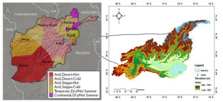
Afghanistan, located in the heart of south-central Asia between 33°56'2.54" N and 67°42'12.35" E (Sarwary et al. 2023), has a semi-arid climate (UNDP 2017; WBG 2021; Rasouli 2022). There is great variation in the climate, soil, topography, vegetation, and natural ecosystems of the country (Aich et al. 2017). Temperature varies greatly by season and altitude, with mountain regions ranging from <0 to >35°C. The average surface air temperature is 13.37°C with a range of 1.92°C, 13.74°C, 24.26°C and 13.41°C in December-February, March-May, June-August, and September-November, respectively. The average annual precipitation is 337.97 mm with a range of 134.35, 146.04, 22.03, and 35.05 mm in December-February, March-May, June-August, and September-November, respectively (WBG 2021).
This study was conducted in Kabul, the capital of Afghanistan, south of the Hindu-Kush mountain range. The climate of Kabul is affected by the climate of the Hindu-Kush mountains. This region has a continental, cold, semi-arid climate with rainfall concentrated in the winter and spring months. Winter (January-March) is a very cold season with snowfall, while spring is more humid with higher precipitation frequency. Summer has very low precipitation; it is the warmest season, with a longer sunshine period of about 356.8 hours per month in July and very low humidity (36% in June). Autumn has low rainfall of 3.7 mm, 18.6 mm, and 21.6 mm for October, November, and December, respectively, with warm afternoons and cool evenings. Kabul is situated at 34.45 N and 69.00 E at an elevation of 1805 m above mean sea level and covers a total area of 4655.25 km2 (Table 1). The local steppe climate influences Kabul, which receives little yearly rainfall. The average annual temperature is 11.4°C, and the annual total precipitation is 362 mm. The driest month is June with about 1 mm of precipitation. Most rainfalls in March average 88 mm. July, with an average temperature of 23.2°C, is the warmest month. The lowest average temperature for the year is –2.9°C in January.
2.2. Data description
2.2.1. Site data
The daily observed maximum (Tmax) and minimum temperature (Tmin) were acquired from the meteorological stations collected by local organizations, including MDA, MAIL, and MEW, from 2003 to 2020 and online data sets. The thirty years of data (1990-2020) were used as the observed data period.
2.2.2. NCEP/NCAR reanalysis data
The daily reanalysis data for the baseline period were acquired from the NCEP/NCAR. NCEP predictors, in the SDSM model, for the relationship among the NCEP predictors and local predictands were applied for screening purposes (Saddique et al. 2019; Munawar et al. 2022). The NCEP/NCAR data were acquired from the GCM (CanESM2) model.
2.3. RCP Scenario Data
The Coupled Model Intercomparison Project Phase 5 (CMIP5) IPCC report that provides a wider picture of future climate change scenarios was used. Three future climate change scenarios, including a mitigation scenario (RCP 2.6), a medium stabilization scenario (RCP 4.5), and an extreme scenario (RCP 8.5) (Saddique et al. 2019) were selected for the periods of 1990-2100. RCPs describe different levels of greenhouse gases and other radiative forcing that might occur in the future. RCP 2.6 leads to a very low forcing level, RCP 4.5 leads to a medium forcing level, and RCP 8.5 leads to very high emission scenarios (Wayne 2013). Trend analysis was conducted by parametric methods such as regression.
2.4. Projection and downscaling
Downscaling of Tmin and Tmax was performed using two models, SDSM and LARS-WG. The available observed data were obtained from MAIL, AMD, and MEW and the missing data were derived from the open-source datasets for the period of 1990-2020.
LARS-WG is a stochastic weather generator that was applied for the simulation of weather data for reference and future climatic variable conditions. The observed climatic data (Tmax and Tmin) were used in LARS-WG to generate time series for future periods. The future climate scenarios were generated for the periods of 2025 -2100 for selected RCPs (RCP 2.6, RCP 4.5, and RCP 8.5) based on the baseline parameters.
SDSM was used to develop the relationship between the predictands (Tmax and Tmin) and NCEP/NCAR predictors. NCEP predictors were used to simulate the time series data for the periods. The performance of the models to generate synthetic time series was calibrated and validated (Saddique et al. 2019; Javadinejad et al. 2021).
2.5. Model performance
Trend analysis was conducted by parametric methods such as linear regression as given by equation 1:
Y = a + bX (1)
where: X is the explanatory variable; Y is the dependent variable; a is the intercept, b is the slope of the line.
The performances of the models were estimated by comparing the observed and generated Tmin and Tmax data by using statistical indicators. These indicators were computed by the equation 2-6 as follows:
R2 = Var-Exp by mod/Total variance (3)
NRMSE = RMSE/Xi (6)
Here: R is the correlation coefficient; R2 is the determination coefficient; MAE is mean absolute error; RMSE is root mean square error; NRMSR is normalized root mean square error; X and Y are the values of variables; and x̄ and ȳ are the means of variables. Xi is the observed value of variables; Yi is the simulated value by the models; and n is the measured number (Ababaei et al. 2010; Delavar et al. 2016; Kounani et al. 2021; Munawar et al. 2022).
3. Results
3.1. Evaluation criteria
The results of the statistical measures proved both models were efficient over the validation period for the variables Tmin and Tmax. Table 2 illustrates measured indices of the statistical downscaling models. The models (SDSM and LARS-WG) were assessed (validated) by using statistical measures: R, R2, MAE, RMSE, and NRMSE (%) between observed and simulated data. The results of statistical measurements proved that both models are efficient for the estimation of Tmin and Tmax, as shown in Table 2.
3.2. Temperature trend analysis for observation data
To analyze the variation of temperature variables for Kabul meteorological stations, daily observed data from local data sets (MAIL 2022; MDA 2022; MEW 2022) were used. The monthly and yearly averages of temperature are shown in Figure 2.
Fig. 2.
The average monthly maximum (Tmax), mean (Tave), and minimum (Tmin) temperatures during the reference period (1990-2020).
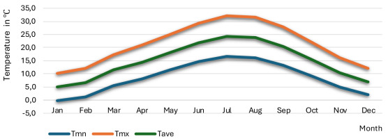
Analysis of average monthly temperature trends indicates that January is the coldest month and July is the warmest month, with a range of –2 to 16.7°C in Tmin, 5.0-24.3°C in average temperature, and 10.2-32.1°C in Tmax.
3.3. Temperature trend analysis for the future
Annual changes were projected for maximum, average, and minimum temperatures under three RCPs for the future (2025-2100). Table 3 shows the projected average temperature during 2025-2100 based on the reference period (1990-2020) under RCP 2.6, RCP 4.5, and RCP 8.5. Moreover, Figure 3 shows the average temperature change compared to the future and baseline periods.
Table 3.
Average annual average temperature during reference (1990-2020) and future (2025-2100) periods.
Fig. 3.
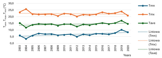
Multi-year sequence (2003-2020) of the average annual maximum (Tmax), annual mean (Tave), and annual minimum (Tmin) temperature.
Average annual maximum temperature was shown in Table 4 and Figure 5 during reference and future periods.
Table 4.
Average annual maximum temperature during reference (1990-2020) and future (2025-2100) periods.
Fig. 4.
The comparison of annual average temperature for the reference and future periods under different RCPs.
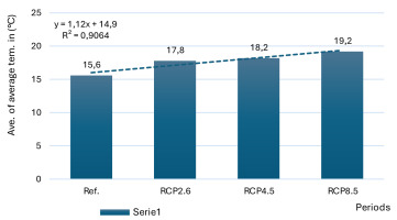
Fig. 5.
The comparison of average maximum temperature for the reference (1990-2020) and future (2025-2100) periods under RCP 2.6, 4.5, and 8.5.
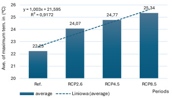
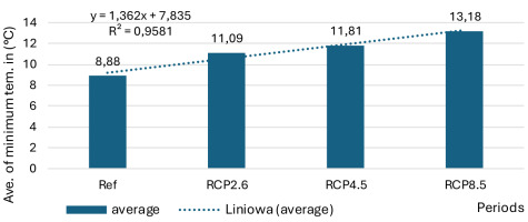
Table 5 and Figure 6 illustrated the average minimum temperature based on reference periods.
Table 5.
Average annual minimum temperature during reference (1990-2020) and future (2025-2100) periods.
Fig. 6.
The comparison of average minimum temperature for the reference (1990-2020) and future (2025-2100) periods under RCP 2.6, 4.5 and 8.5.
The annual change in temperature trends (average, maximum, and minimum temperature) is shown in Tables 6-8. Table 9 shows the monthly change in temperature trends. Table 9 shows the change in temperature trends by month (maximum, average, and minimum temperature) over the projection period (2025-2100)
Table 6.
Annual changes of maximum temperature during the projection period (2025-2100) under RCP 2.6, RCP 4.5, and RCP 8.5.
| Annual change in maximum temperature (°C) | |||
|---|---|---|---|
| RCP2.6 | RCP4.5 | RCP8.5 | |
| 2025 | 1.3 | 1.6 | 1.8 |
| 2030 | 1.4 | 1.2 | 1.5 |
| 2040 | 1.1 | 1.1 | 1.4 |
| 2050 | 2.0 | 2.4 | 3.1 |
| 2060 | 1.8 | 2.2 | 2.9 |
| 2070 | 2.1 | 3.5 | 4.9 |
| 2080 | 1.9 | 3.3 | 4.8 |
| 2090 | 2.2 | 3.6 | 6.3 |
| 2100 | 2.7 | 4.0 | 6.8 |
| Avg. | 1.8 | 2.5 | 3.7 |
Table 7.
Annual change in average temperature during the projection period (2025-2100) under RCP2.6, RCP4.5 and RCP8.5.
| Annual change in average temperature (°C) | |||
|---|---|---|---|
| RCP2.6 | RCP4.5 | RCP8.5 | |
| 2025 | 1.2 | 1.1 | 1.4 |
| 2030 | 1.2 | 1.4 | 1.7 |
| 2040 | 1.5 | 1.5 | 2.0 |
| 2050 | 2.1 | 2.4 | 3.2 |
| 2060 | 2.1 | 2.5 | 3.3 |
| 2070 | 2.1 | 3.4 | 5.1 |
| 2080 | 5.0 | 3.5 | 2.2 |
| 2090 | 2.2 | 3.6 | 6.3 |
| 2100 | 2.9 | 3.9 | 7.0 |
| Ave. | 2.2 | 2.6 | 3.6 |
Table 8.
Annual change in minimum temperature during the projection period (2025-2100) under RCP 2.6, RCP 4.5 and RCP 8.5.
Table 9.
Changes in temperature trends by month (Tmin, Tmax, and Tavg) under RCP 2.6, RCP 4.5, and RCP 8.5 over the period 2025-2100.
The monthly projected Tmin showed an increase ranging between 2.38°C, 3.20°C, and 4.61°C under RCP 2.6, RCP 4.5, and RCP 8.5, respectively. The monthly projected maximum temperature showed an increase ranging between 1.88°C, 2. ° C, and 3.92°C under RCP 2.6, RCP 4.5, and RCP 8.5, respectively. Also, the monthly projected average temperature showed an increase ranging between 2.13, 2.92, and 4.26°C under RCP 2.6, RCP 4.5, and RCP 8.5, respectively. The results showed a continuously increasing trend of projected temperature in future scenarios.
4. Discussion and conclusion
This study was carried out to estimate temperature variables in the reference (1990-2020) and future (2025-2100) periods under RCP 2.6, RCP 4.5, and RCP 8.5 by using two statistical downscaling models (SDSM and LARS-WG). In general, according to the performance indicators, both models (SDSM and LARS-WG) are efficient for downscaling and projecting, but the LARS-WG model was approximately more suitable. The temperature trends (minimum, maximum, and average temperature) are shown to increase by a range of 0.28°C, 0.69°C, and 0.48°C, respectively the reference period (1990-2020).
The future temperature is predicted to increase from 2025 to 2100 at much higher rates compared to the reference period, under three RCPs. Average temperature showed an increase under RCP 2.6, RCP 4.5, and RCP 8.5 of 2.3°C, 2.6°C, and 3.6°C, respectively. Average temperature would increase by 12.9%, 14.3%, and 18.8% (Table 3, Fig. 4) by 2100 under RCP 2.6, RCP 4.5 and RCP 8.5, respectively. Maximum temperature would increase under RCP 2.6, RCP 4.5, and RCP 8.5 by 1.8°C, 2.5°C, and 3. ° C, respectively, for the future periods. Maximum temperature would increase by 7.7%, 10.3%, and 14.3% under RCP 2.6, RCP 4.5, and RCP 8.5, respectively, by 2100 compared to the reference period. Moreover, an increase in annual minimum temperature by 2100 was predicted at 2.2 C, 2.9 C, and 4.3 C under RCP 2.6, RCP 4.5, and RCP 8.5, respectively. The minimum temperature would increase at a rate of 19.9%, 24.9%, and 32.7% (Table 5, Fig. 6) under RCP 2.6, RCP 4.5, and RCP 8.5, respectively, during 2025-2100. Temperature increases with a range of values have been reported in many studies, such as Aich et al. (2017), Hassanyar et al. (2017), UNDP (2017), and WBG (2021). A 1°C increase from 1900-2017 was reported in WBG (2021). Annual temperatures have also been projected to increase by 3.50°C and 7.00°C (NEPA 2018), or 1.70°C and 2.30°C (Sarwary et al. 2023) by 2050; increases of 2.00°C and 6.50°C (FAO 2016) or 2.70°C and 5.50°C (WBG 2021) by 2100 under RCP 4.5 and RCP 8.5, respectively, relative to the baseline period in Afghanistan. The temperature increase was projected to occur most rapidly during spring and summer at higher altitudes (central highlands and Hindu Kush) (NEPA 2018). Moreover, an increase in global mean temperature by 0.30-1.70°C under RCP 2.6, 1.10-2.60°C under RCP 4.5, and 2.60-4.80°C under RCP 8.5 has been projected by the end of the 21st century (2081-2100) relative to 1986-2005 (IPCC 2014). The global mean temperature is expected to increase by 1.40-5.80 C by 2100 (Sarwary et al. 2023).
This study revealed that temperature trends increase during reference and future periods. Climatic variation can affect many aspects of environmental systems. Although this study highlights temperature trends, additional climatic factors such as precipitation, wind speed, and solar radiation need further study. An increase in temperature would affect ecosystems, agricultural production, human health, and more environmental systems.
Afghanistan has faced a higher increasing temperature than the global average over the century, and it shows extreme vulnerability to hazards such as drought and flood. Findings revealed that an increase in temperatures (average temperature and maximum temperature) harms wheat production because of heat and drought stress, while the increase in minimum temperature has a positive effect on wheat production. This vulnerability is amplified by poverty, undernourishment, food insecurity, and inequality. These are the driving forces of negative impacts on agriculture, natural resources, natural ecosystems, forests, water resources, and society.

