1. Introduction
Estimating the most precise possible rating curve is one of the main and most difficult tasks facing contemporary hydrology. The problem is of fundamental importance for the prediction of flood events, rational use of water resources, the design of hydro-technical structures, where extreme flow rates are accepted as the design standard (Ozga-Zieliński et al. 2014), and the determination of flood-threatened zones based on maximum flows and the corresponding stages (Radczuk et al. 2001). The rating curve is also the basis for the determination of hydrological criteria (Eagelson 1978), i.e., seasonal average and extreme flows and time series for estimating the response of the catchment basin at high and low water stages. A correctly plotted rating curve can also be a reference for estimating maximum annual flows (Szulczewski et al. 2018).
The problem of precise estimating of the rating curve has been addressed previously in numerous publications and monographs. The uncertainty of rating curves arises from two sources (Westerberg, McMillan 2015). First are the hydrometric measurements from which the curve is plotted. The accuracy of measurements is extremely important for estimating a good rating curve, and errors in river flow data are far from negligible (Di Baldassarre, Montanari 2009). The second source, usually more important, is precision in the determination of the relationship between the discharge and the stage. Errors resulting from both of those sources have been analyzed with various methods in numerous studies. Lang et al. (2010) propose the use of Bayesian methods in combination with the Markov Chain Monte Carlo (MCMC) process for analyzing the problem. In that study, as background for advanced analysis, historical measurements were analyzed to identify errors resulting from inaccurate measurements and changes in the cross-section of channels. The advanced analyses were conducted on a suitably reduced data set. We can, therefore, consider partial homogenization of the analyzed data. Conclusions following the study by Lang et al. (2010) indicate that a lack of analysis of errors in rating curves can result in inaccuracies in the estimation of curves. The extrapolation itself is already burdened with inaccuracy. Reitan and Petersen-Overleir (2009), using similar methods, propose the estimation of a segment curve which provides better accuracy for those flow regimes at which measurements are seldom taken.
Interpreting the rating curve, especially in the case of estimating flood risk, should account for potential errors of estimation (Singh, Strupczewski 2002; Haque et al. 2014).
The goodness of fit of rating curves can be tested with a variety of indicators. A comparison of eleven such indicators is presented in the paper by Krause et al. (2005). The authors demonstrate that the most frequently applied indicators of fit may not give the best results, and even high values do not necessarily mean a good-fitting curve.
The rating curve is a non-linear function H = f (Q) describing the relation between the stage H and the discharge Q. It is plotted based on hydrometric measurements, which, due to their level of precision, can be one of the sources of its uncertainty (Domeneghetti et al. 2012). The curve can be plotted and described with the use of various formulae and methods. Frequently applied formulae include, e.g., the Chezy and Manning formulae, which relate the mean water flow rate in a profile with tangent stress in a wetted perimeter (Strupczewski 1996; Fenton, Keller 2001). Those formulae work well in the case of monotonic flow in an open channel. A study by Leonard et al. (2000) indicates that such an approach can be successfully applied in the case of rivers with variable sections. Direct application of the Chezy and Manning formulae, however, can be tedious due to the number of parameters. In addition, some of the variables are determined separately for channel water and flood areas, and others in a descriptive manner (Szkutnicki et al. 2007). Incorrect interpretation of any of the parameters results in an erroneous evaluation of the flow value.
A more universal formula is the Harlacher formula (Byczkowski 1999) which relates the stage of water directly with the volume of flow at the given cross-section. In addition, the Harlacher formula describes the opposite relationship, Q = f (H), which simplifies calculations and the interpretation of results. This formula is expressed as:
Q = α (H – B)n
where α and n are parameters, and B is the state of zero flow (Szkutnicki et al. 2007). The constant B can be determined from the cross-section of the bottom or the longitudinal profile of the watercourse, or with graphical and graphical analytical methods Dębski (1955); Byczkowski (1999). In practice, however, it is most often assumed that B = 0. With that assumption, the rating curve equation has the following form:
Q = aHb (1)
where a and b are parameters. The literature (Dębski 1955; Szkutnicki et al. 2007) proposes the determination of parameters a and b through the linearization of Eq. 1 by using a logarithmic model. A rating curve based directly on parameters determined in this manner is easy to interpret, and its shape is uniquely described by the shape of the channel profile (Ozga-Zieliński et al. 2014). The logarithmic curve, however, does not provide the required accuracy because of widely scattered data. A comparison of the logarithmic method of rating curve determination with historical methods based on fitting quadratic and cubic polynomials to the data is presented by Sivapragasam and Muttil (2005). Their study indicates that the results obtained with conventional methods can be improved by means of the alternative approaches to the problem that they propose. Sivapragasam and Muttil (2005) determined the stage-discharge relationship using the SVM (Support Vector Machine) and ANN (Artificial Neural Network) methods. Those methods, however, given their complexity, are still difficult to apply in operational use. Another alternative method for estimating the rating curve is proposed by Dottori et al. (2009). It is based on a parabolic differential equation relating the lowering of the water level in the channel to local and convective acceleration in the stream. The proposed method gives very good results and allows the extrapolation of the curve in cases when there is a lack of measurements in the high discharge zone.
All of the studies mentioned above were conducted on hydrometric data collected during multi-year measurement series. In most cases, there is no information as to whether the data had been transformed in any way before the analyses. One can assume, therefore, that they did not constitute homogeneous sets. Non-homogeneity of measurement data can have numerous causes. It can result from a change of the measurement site, as in the case described above, but also, e.g., from a change in the method of data acquisition, movement of the water gauge to another location, change of ordinate ”0” of the water gauge, or from other anthropogenic and natural factors (Ozga-Zielińska, Brzeziński 1994). The problem of non-homogeneity was also noted by Szulczewski and Jakubowski (2018). Those authors indicate that a more accurate analysis of data sets can be performed by assuming a priori their non-homogeneity and applying a mix of two different probability distributions for their description.
The objective of this paper is to propose a method for homogenizing a set of hydrometric measurements based on the location of measurements.
2. Data and methods
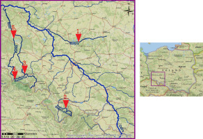
The analyses were conducted on measurement data provided by the Institute of Meteorology and Water Management, State Research Institute. The hydrometric data obtained related to rivers and cross-sections that were selected as representative of mountain, submontane, and lowland rivers. Table 1 is a compilation of information on the selected cross-sections. The selected stations are marked in Figure 1. The hydrometric measurements included such features of the watercourse as the water stage H [cm], discharge Q [m3/s], average and maximum velocity Vavg and Vmax [m/s], area of wetted cross-section F [m2]. The discharge is calculated from the measured average flow rate. The data tables also include information on the distance from the water gauge [m] and the direction relative to it from which the measurement was taken.
Table 1.
Selected representatives of river types. H = water stage, Q = discharge, F = area of wetted cross-section, Vavg = average flow velocity, Vmax = maximum flow velocity.
Based on data from the individual water gauge profiles, rating curves were plotted per Eq. 1. Parameters a and b were calculated with a non-linear regression model. The goodness of fit of the curves to the data sets was described with the Nash-Sutcliffe index:
where Qm means the theoretical value of discharge volume calculated from Eq. 1, Qo is a value observed in measurements, and
Fig. 1.
The region analyzed shown on the map of Poland. Locations of cross-sections selected for analysis: 1 – Barycz, Łąki; 2 – Biała Lądecka, Lądek Zdrój; 3 – Bóbr, Jelenia Góra; 4 – Kamienna, Jakuszyce; 5 – Kwisa, Łozy. Source: National Geographic ESRI Garmin Map.
Referring to the study by Krause et al. (2005), the index NSE was compared with two other measures of the goodness of fit. One of them, proposed by the authors of the cited study, is the modified form of that index, called the relative index NSErel. It is characterized as follows:
where the symbols and the interpretation of the resulting value are the same as in the case of the classic NSE. The other measure is the relative mean error of fit ηrel, defined as:
Low values of coefficient ηrel indicate a good fit of the rating curve to the data set.
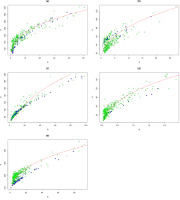
Significant sources of non-homogeneity of data sets include, e.g., the place where the measurement was taken and the method with which it was made (Bartnik, Jokiel 1997). The literature provides numerous comparisons of methods of measurement with the use of the current meter and, acoustic Doppler current profiler (ADCP; Delcroix et al. 1992; Hayes et al. 2012; Chauhan et al. 2014), and detailed descriptions of those methods (Gore, Banning 2017), but there is no model that would permit homogenizing data in relation to the method of measurement. Figure 2 presents hydrometric data limited to measurements taken at medium and low stages at selected cross-sections, with the method of measurement indicated. In a majority of cases, except for the measurements taken on the Barycz River (a lowland river), one can observe a distinction between the appearance of the two groups related to the method with which the measurements were taken. Due to the substantial non-homogeneity of the data resulting from the methods of measurement, we decided to use only the results from current meter measurements for this study. Data acquired with the current meter method are abundantly represented at each of the given cross-sections. In addition, at high stages on the mountain rivers, the measurements are taken with that method only, therefore, the acquired information is used for the approximation of the rating curve describing high water stages. For this study, we also decided to use all of the measurements (both historical and the latest) to increase the number of observations. The method was conducted on other, smaller data sets from short periods of time to satisfy the assumption that the river shape was constant, as it would not be over long periods of time (Domeneghetti et al. 2012). The distances between a given point of measurement and the given cross-section proved to be highly diverse. Approximately 50% of the measurements were taken exactly in the given cross-section, but the other measurements were taken at a smaller or larger distance (from several to several hundred meters) from the given cross-section, both upstream and downstream. This variation in distances of hydrometric measurements from the given cross-sections motivated the construction of a transformation allowing partial homogenization of measurement data. The transformation was based on the assumption of constant discharge in time at a given measurement, irrespective of the point at which it was taken. When the velocities are measured away from the given cross-section, and the discharge is calculated based on their values, the stage values are taken from the water gauge profile. Upon application of the transformation, stages that would appear on the cross-section at such discharges were assigned to the discharges from measurements taken away from the given cross-section. Since the discharge is constant, for the transformation, the changes in the river geometry were left out. The first step of the transformation was the estimation of the rating curve for the data acquired in the given cross-section,
Fig. 2.
Hydrometric data for medium and low stages from selected cross-sections. Green: data acquired by current meter; blue: data acquired by ADCP; open dots: data acquired with other methods; (a) Barycz, Łąki; (b) Biała Lądecka, Lądek Zdrój; (c) Bobr, Jelenia Góra; (d) Kamienna, Jakuszyce; (e) Kwisa, Łozy.
The data corresponding to the measurements taken outside of the given cross-section were divided into two groups, one acquired downstream and the other upstream from the cross-section. The rating curve
where the index 0 denotes the group of measurements taken in the given cross-section, and the index 1 indicates measurements outside of the profile.
Next, the two groups were transformed separately to the given cross-section per Formula 5. For the transformed data, a new rating curve was plotted, using the non-linear least squares method. The fit of the curve to the data set was described by the indices NSE, NSErel, and ηrel in conformance with 2, 3, and 4.
3. Results and discussion
Table 2 presents the values of the parameters of fit (NSE, NSErel, and ηrel) for the data, both before and after the transformation. In most of the cases analyzed, the rating curve was a slightly better fit to the data after the application of the transformation than before it. However, the differences in most of the parameters are <1%, and, therefore, can be treated as negligible. A greater difference in the parameter ηrel in favor of no transformation (>3%) was observed for the water gauge Łąki on the Barycz River. According to Krause et al. (2005), however, the measures of fit can be doubtful, and consequently, small differences in the values of the parameter may be insignificant. Thus, we conclude that in the cases analyzed, transformation of the measurement data did not improve the fit of data to the rating curve.
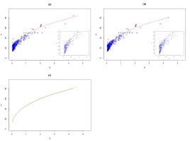
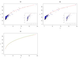
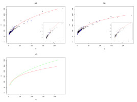
Figures 3-7 present the relationship Q = f (H) for the selected representatives of mountain, submontane, and lowland rivers. A difference was observed in the layout of points representing measurements on a plane. In the low stages zone, the scatter of measurement points decreased after the transformation. This result is of great importance in the plotting of the rating curve, as it allows a single description for all measurements from that zone. The transformation also had an impact on the zone of high stages. Because of the difficulties involved in taking measurements at high water stages, that group is never well represented, and therefore even a slight shift of data causes a big difference in the shape of the rating curve, and consequently, either an overestimation or underestimation of the discharge. Parts (a) and (b) of each of the figures illustrate data before and after the transformation, respectively, with the fitted rating curves. In the right bottom corner of every graph, there is an enlarged area of low water stages. Blue indicates measurements taken in the water gauge profile, i.e., those that were not transformed. Part (c) is a comparison of the fitting of the rating curve before and after the transformation. Green is used for the curve corresponding to non-modified data. Red is used for the curve fitted to the data after the transformation. This makes it easier to notice the differences in the shapes of the curves.
Table 2.
Measures of rating curve fitting error.
In the case of the water gauge Łąki on the lowland Barycz River, the transformation had only a slight effect on the distribution of the data and the fitting of the rating curve. The values of the indices NSE and NSErel differ at the level of thousandths (<1%) in favor of the transformation, and the relative error ηrel points in favor of no transformation. Differences of this magnitude are insignificant. The differences in the shapes of the curves can be observed in Figure 3c. The curve fitted to the data after the transformation indicates a possibility of somewhat higher stages for high discharge volumes. In the zone of low stages, the rating curve after the transformation is slightly more flattened relative to the initial curve.
Significant changes in the fitting of rating curves to the data after the transformation can be observed in the next two cases analyzed. Figure 4 presents the effect of transformation of data from the water gauge Lądek Zdrój on the Biała Lądecka River. In the zone of low-water stages, a relatively large number of measurements were taken exactly in the water gauge profile, and hence for low discharge volumes, the difference between the curves before and after the transformation is small. In the zone of high-water stages, in which measuring strictly at the water gauge is often impossible, one can observe a notable difference in the shapes of the curves. No transformation of the data can result in a big underestimation of the level of the high water stage. In addition, the indices NSE, NSErel, and ηrel imply a difference in the goodness of fit in favor of the curve plotted with the transformed data. Similar observations can be made in the case of the water gauge station Jelenia Góra on the Bóbr River (Fig. 5). Also, in this case, all of the parameters indicate a better fit of the curve after the transformation of the measured data. The rating curve for the zone of high-water stages for the data before the transformation is overestimated relative to the curve for the transformed data. In addition, one can note how important it is to take measurements directly in the water gauge profile at low-water stages. The rating curves for data before and after the transformation are divergent also in the zone of low-water stages, i.e., in the zone where the relatively largest number of measurements are made.
In the case of the water gauge station Jakuszyce on the Kamienna River (Fig. 6), we can observe a nearly perfect coincidence of the curves before and after the transformation. This attribute results from the precision of the measurements; only a few of them were taken outside of the water gauge profile. The small difference in the goodness of fit of the curves described by the index ηrel results from a slight shift of the measurements taken outside of the water gauge profile in the zone of low-water stages.
In the case of the water gauge station Łozy on the Kwisa River (Fig. 7), the parameters indicate an almost identical level of goodness of fit of the curves to the data sets. Although the majority of the measurements were taken outside of the water gauge profile, the curves differ slightly only in the zone of high-water stages.
Fig. 3.
Rating curve for the Barycz River at water gauge station Łąki; (a) before transformation, (b) after transformation, (c) comparison of rating curves before (green) and after (red) transformation.
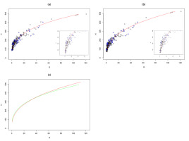
Fig. 4.
Rating curve for the Biała Lądecka River at water gauge station Lądek Zdrój; (a) before transformation, (b) after transformation, (c) comparison of rating curves before (green) and after (red) transformation.
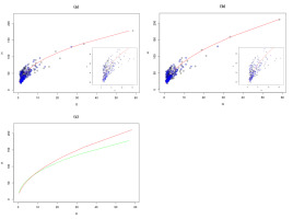
Fig. 5.
Rating curve for the Bóbr River at water gauge station Jelenia Góra; (a) before transformation, (b) after transformation, (c) comparison of rating curves before (green) and after (red) transformation.
4. Conclusions
The differences between the rating curves for the transformed and untransformed data are greater for rivers on which hydrometric measurements were taken at various and large distances from the water gauge profile. The type of watercourse is also important; measurements from the mountain and submontane rivers, characterized by a greater range of both medium and high flow velocities (as per Table 1) and large variations of cross-section, even over short distances, are more sensitive to the application of the transformation. This means that, especially in the case of rivers of this type, the most accurate rating curve can be obtained by taking hydrometric measurements directly in the water gauge profile.
With automated tools and analytical methods, one can relatively easily fit a curve to a selected data set. The problem appears when a data set is not homogeneous, as then it is not possible to treat all of its elements in the same way. The proposed transformation homogenizes the hydrometric data relative to the place of measurement.
The pre- and post-transformation rating curves fit the data similarly. Small differences in the values of the indices NSE, NSErel, and ηrel can be considered negligible. The similar values indicate that the proposed method fits the rating curve to the data set well, and the transformation does not affect the quality of this fit. The transformation, however, has an impact on the distribution of measurement points both in the zone of low-water stages and in that of high stages. The differences affect the inference and the prediction of discharge rates. Precise determination of the stage-discharge relationship is very important for accurate evaluation of the behavior of catchment basins under various hydrological conditions.
The transformation eliminates one of the sources of inhomogeneity in the hydrometric data, which permits analyses of a partially homogeneous data set. Striving to homogenize data sets at successive levels, for example, to adjust for the measurement method, may consequently lead to simplification of the methods and interpretation of the results of the analyses.
The natural characteristics of watercourses, such as overgrowing, which are not included in the transformation, deserve special attention. These phenomena can have significant impacts on the precise determination of rating curves, especially in lowland rivers.

