Identification of nominal release policies implemented in a multi-purpose water reservoir

A water reservoir’s operation should follow a rational policy to ensure adequate water provision for different purposes without adverse effects. However, it is not well-studied how to identify operational policies currently being implemented. This study establishes a new approach to identifying nominal release policies as implemented in a multi-purpose water reservoir. We chose Bukit Merah Reservoir (BMR), located in Perak State, Malaysia, as a study site to examine its release policies for meeting irrigation, municipal, and industrial water demands and for mitigating floods and environmental hazards. The operator of BMR releases the reservoir’s water into two primary irrigation canals, the Main Canal and the Selinsing Canal. Generalized additive models (GAMs) are applied to time series data observed at BMR to identify the annual dynamics of its water management. Operational policies for the release discharges into the two primary irrigation canals are assumed to be based on information on the time-of-year and the reservoir water level. First, a backfitting algorithm identifies each contributing function of the GAMs representing the release policies. Then, spurious oscillations in the functions are removed by total variation (TV) regularization (TVR) to obtain nominal release policies, which are quite reasonable in the sense of conventional reservoir management practice. Finally, the identified nominal release policies are utilized to examine shifts in the operation of BMR during the period from 2000 through 2011. The decomposition of release policies illustrates the two aspects of the irrigation demand’s annual patterns and the hydraulic structures’ functions. The spurious oscillations removed by TVR are considered to represent indecision by the reservoir operator.

1. Introduction

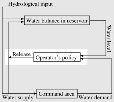
In recent decades, climate change and socio-economic growth have had impacts on available water resources and food security in most parts of the world (Biemans et al. 2013; Lee, Bae 2015). Thus, more sophisticated management of existing water resources (Mereu et al. 2016; Wałęga et al. 2020), environments (Alam et al. 2018), and ecosystems (Yaegashi et al. 2018) is required to adapt to the impacts. A water reservoir’s operation should follow a rational policy to ensure adequate water provision for its various intended purposes without adverse effects. Figure 1 shows a conceptual diagram of a typical reservoir operation system in the context of feedback control theory. Hydrologic inputs, including precipitation, evapotranspiration, and runoff from the catchment, affect the reservoir’s water balance and the water supply to the command area (i.e. the downstream area serviced by the reservoir’s functions). The release from the reservoir as a control variable also contributes to the reservoir’s water balance and the water supply to the command area. The operator’s role is to implement a policy determining the release discharges based on the reservoir’s water level and the water demand from the command area. However, a more sophisticated system of reservoir operation might also account for hydrologic inputs and/or possible conveyance losses as parts of the information on which the policy is based.

Fig. 1.

Conceptual block diagram of a reservoir operation system.

http://www.mhwm.pl/f/fulltexts/154592/MHWM-9-0010-g001_min.jpg

Labadie (2004), Rani and Moreira (2010), and Ahmad et al. (2014) reviewed a variety of methods for computationally determining suitable reservoir operation policies. Stochastic dynamic programming (SDP) theory is the general framework to establish reservoir operation policies, as explored decades ago (Heidari et al. 1971; Tejada-Guibert et al. 1993, 1995; Yakowitz 1982). The SDP typically provides optimal operation policies with thresholds of opening valves or switching pumps (Nop et al. 2021; Unami, Mohawesh 2018; Unami et al. 2019b). However, reservoir operators generally do not accept such theoretically generated policies but instead rely on their empirical knowledge to make decisions when unexpected risks are involved (El-Shafie et al. 2014). Therefore, attention should be paid to the actual policies that may be identified from historical data (Giuliani et al. 2014). Turner et al. (2021) firstly attempted to inventory reservoir operation policies in the United States.

This study aims at establishing a new approach to identifying nominal release policies implemented in a multi-purpose water reservoir. Bukit Merah Reservoir (BMR), located in the northern part of Perak State, Malaysia, was chosen as a study site. The water levels and release discharges of BMR were recorded daily from 2000 through 2011. Generalized additive models (GAMs; Chen, Tsay 1993) are applied for representing the operational policies for release discharges, which are assumed to have an annual period based on the day of the year and the water levels (Unami et al. 2019a). The backfitting algorithm works well to identify each contributing function of the GAMs (Breiman, Friedman 1985). However, the release policies identified with that method include spurious oscillations, which are removed with total variation regularization (TVR), known as the Rudin–Osher–Fatemi model (ROF) for the initials of its three authors (Rudin et al. 1992). The ROF model contains a scale parameter dominating the discrepancy of the reconstructed data from the original data that includes spurious oscillations (Osher et al. 2005). Further application of TVR in agricultural water management was discussed in Fadhil and Unami (2021). The identified release policies, which are considered nominal because they have been smoothed and regularized, are utilized to examine shifts in the operation of BMR during the period. Several factors stemming from climate change and socio-economic growth are inferred to have burdened the operation of BMR with more demanding release policies.

2. Materials and methods

2.1. Study site and datasets

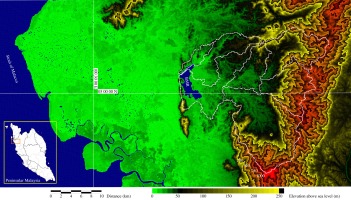
Figure 2 shows the topography of BMR’s catchment and command areas, extracted from the Shuttle Radar Topography Mission (SRTM) digital elevation data (Farr et al. 2007), with the boundaries of sub-catchments demarcated with white lines. The climatic zone is tropical rainforest with a mean annual rainfall of more than 3000 mm. The bimodal annual rainfall pattern enables paddy rice cultivation twice a year. BMR has a catchment area of 480 km²; it supplies irrigation water to the paddy fields of the Kerian Irrigation Scheme (KIS), covering an area of 236 km², and urban water for municipal and industrial purposes to the Kerian, Larut, Matang, and Selama Districts. The catchment includes four river systems: Merah, Jelutong, Selarong, and Kurau Rivers (Ismail, Najib 2011), located between 04 51 N and 05 10 N latitude and 100 38 E to 101 00 E longitude. The region is primarily rural with numerous riverine villages established along the middle and lower reaches of the rivers. The land use in the areas with elevations lower than 50 m is predominantly for tree plantations such as oil palm, rubber, and coconut. At the same time, the surrounding steep mountain slopes are covered with rainforests. The rainfall characteristics in the catchment area have been modeled with a stochastic generator (Fadhil et al. 2017). Analysis using rainfall-runoff models with fractional derivatives has shown that the hydrologic response in the catchment area of the Kurau River is unstable (Unami et al. 2021). The KIS’s 236 km² command area consists of low-lying lands between the Strait of Malacca and BMR. Two primary irrigation canals, the Main Canal and the Selinsing Canal, convey the irrigation water by gravity. The urban water is taken from the Selinsing Canal at a pumping station located 6.5 km downstream of BMR. Dor et al. (2011) conducted a detailed hydro-geological study on the Selinsing Canal. Approximately 61% of water consumed in the paddy fields of the KIS originates from BMR, and the rest is from rainfall (Hamidon et al. 2015). Urban demand depends on the local population and its economy. The Department of Irrigation and Drainage (DID, 2011) projected that the growth rates of the population and economy in the state of Perak would decrease but remain positive until the year 2050. Intensive research on the operation of BMR has been conducted in the context of future climate change and SDP (Fadhil 2018). Besides the irrigation and urban demands, the operation of BMR needs to account for flood control and environmental hazards. There are two gated spillways of Ogee weir type with the same crest level, draining water from BMR to the original water course of the Kurau River, which meanders through the KIS with widths of 30-50 m.

Fig. 2.

The topography of the catchment and command areas of BMR, located in Peninsular Malaysia.

http://www.mhwm.pl/f/fulltexts/154592/MHWM-9-0010-g002_min.jpg

The key dimensional parameters of BMR are summarized in Table 1. The dam embankment is at an elevation above the sea level (EL) of 11.28 m. The datum level is taken as the lowest level of the reservoir. The water level above the sea level is denoted by h (m). The storage volume of the reservoir when the water level is equal to h is denoted by V(h). The maximum capacity of the spillways at MWL is 565 m³/s. However, the bed slope of the Kurau River receiving the water from the spillways is about 1/10,000, implying insufficient discharge capacity.

Table 1

Key dimensional parameters of BMR.

Parameter	Description
Maximum water level (MWL) H (m)	EL 10.25
Flood control level (FCL) η_F (m)	EL 9.75
Normal water level (NWL) η_N (m)	EL 8.69
Spillway crest level (SCL) η_S (m)	EL 8.14
Intake gate crest level (IGL) η_G (m)	EL 6.10
Datum level η₀ (m)	EL 2.00
Storage volume (10⁶ m³)	V(h) = 0.190 (h – η₀)^3.17

A daily log of the operation of BMR in terms of water levels, rainfall depths, and release discharges into the two primary irrigation canals for the period from 2000 through 2011 was provided from the DID. The complete source data are available in a supporting information file.

Hamidon et al. (2015) estimated the irrigation demand Q_irr in the KIS for each month. The urban demand Q_urb was assumed to be constant at 1.70 m³/s (Anwar 2010). Then, the sum of the irrigation demand Q_irr and the constant urban demand Q_urb becomes the total demand discharge Q_D for each month. Table 2 summarizes the average monthly rainfall depths R during 2000-2011, the values of Q_irr, Q_urb, and Q_D, and the observed average monthly release discharge Q_R. However, it is noteworthy that the actual irrigation demand varies on a daily scale, according to the GIS-based estimation by Rowshon et al. (2003a-b).

Table 2

Monthly parameter values relevant to the water balance of BMR.

Parameter	Jan	Feb	Mar	Apr	May	Jun	Jul	Aug	Sep	Oct	Nov	Dec
Rainfall depth R (mm)	243.0	174.8	294.3	305.5	155.0	163.1	170.3	215.6	296.9	406.3	356.6	266.8
Irrigation demand Q_irr (m³/s)	11.35	0.39	13.99	15.63	14.95	13.63	10.12	0.35	11.54	12.23	12.54	12.84
Urban demand Q_urb (m³/s)	1.70	1.70	1.70	1.70	1.70	1.70	1.70	1.70	1.70	1.70	1.70	1.70
Total demand Q_D (m³/s)	13.05	2.09	15.69	17.33	16.65	15.33	11.82	2.05	13.24	13.93	14.24	14.54
Observed average release discharge Q_R (m³/s)	5.74	4.18	24.07	28.91	27.18	13.86	4.06	2.79	23.32	29.88	28.52	14.92

2.2. Generalized additive models for release discharges

The water level of BMR at the beginning of day t is denoted by h_t. The release discharge into the primary irrigation canal k on the day t of the year y is denoted by Qy,tk. Here, k = 0 and k = 1 indicate the Main Canal and the Selinsing Canal, respectively. It is assumed that the operator’s nominal policy uk (t, h_t) for release discharge into canal k, based on the information of t and h_t, is yearly invariant. We introduce an additive decomposition structure into uk (t, h_t) to write it as a GAM:

(1)

uk(t,ht)=ftimek(t)+fWLk(ht)+Ck

where ftimek and fWLk are functions that may be nonlinear, and C^k is a constant. Representing the day t as:

(2)

t=2πThedayoftheyear−1Thenumberofdaysin⁡theyear,

the function ftimek is assumed to be 2π-periodic. The objective here is to determine the functions ftimek and fWLk minimizing the errors:

(3)

εy,tk=Qy,tk−ut(t,ht)

in the sense of the least squares as well as the TV.

2.3. Backfitting algorithm

Firstly, the backfitting algorithm is applied for finding the functions to minimize the expected square error E[εt,yk]2 for all the observed data. The algorithm iteratively updates smoothing estimates f^timek and f^WLk of ftimek and fWLk, respectively. Histograms ϕtimek and ϕWLk are defined as:

(4)

ϕtimek(l)=1|Ωt(l)|∑t∈Ωt(l)f^timek(t),Ωt(l)={t|t∈(lΔt−Δt2,lΔt+Δt2)}

and

(5)

ϕWLk(l)=1|Ωh(l)|∑ht∈Ωh(l)f^WLk(ht),Ωh(l)={ht|ht∈(lΔh−Δh2,lΔh+Δh2)}

for integers l with the increments Δt and Δh, respectively. Then, with initial guesses f^timek=f^WLk=0 for all t and h_t, the histograms are utilized to update the smoothing estimates as:

(6)

f^timek(t)=Qy,tk−QWLk(l)−Ck,t∈(lΔt−Δt2,lΔt+Δt2]

and

(7)

f^WLk(ht)=Qy,tk−ϕtimek(l)−Ck,ht∈(lΔh−Δh2,lΔh+Δh2]

where C^k are taken as the averages of all Qy,tk. This algorithm is known to converge under appropriate conditions.

2.4. TVR

After the backfitting algorithm has converged, the TVR is applied to each f^timek and f^WLk=0 to remove spurious oscillations. The TVR operated for a generic oscillating function f over a domain Ω of x minimizes the functional J of u:

(8)

J=∫Ω|∇u|dΩ+λ2∫Ω|u−f|2dΩ

where λ is the scale parameter of the ROF model, and ∇ = ∂/∂x. The Euler-Lagrange equation for minimization of J in (8) is formally written as:

(9)

∇⋅(∇u|∇u|)+λ(f−u)=0.

We attempt to obtain an approximate solution to (9) by numerically solving the initial value problem of the singular diffusion equation:

(10)

∂u∂t=∇⋅(∇u|∇u|)+λ(f−u),u=fatt=0

It is assumed that the values of f are determined at n different points of Ω. Let those points be x_i for i = 0, 1, …, n – 1 such that x₀ < x₁ < … < x_n–1. Applying the standard Galerkin finite element scheme with piecewise linear bases to (10) results in the initial value problem of the ordinary differential equation:

(11)

dudt=M−1Aσ+λ(f−u),u=fatt=0

where u ∈ ℝⁿ is the vector whose i^th entry is u⌢ι, which is the approximation of u at x_i, f ∈ ℝⁿ is the vector whose i^th entry is f at x_i, σ ∈ ℝⁿ⁻¹ is the vector whose i^th entry is the sign of u⌢i+1−u⌢i, M ∈ ℝ^n×n is the mass matrix, and A ∈ ℝ^n×(n−1) is the stiffness matrix. Two types of boundary conditions are considered: periodic and Neumann. For the periodic boundary condition, the matrices become:

(12)

M=(x1−xn−13x1−x060⋯⋯0x0−xn−16x1−x06x2−x03x2−x16⋱⋱⋱00⋱⋱⋱0⋱⋮⋮⋱xi−xi−16xi+1−xi−13xi+1−xi6⋱⋮⋮⋱0⋱⋱⋱00⋱⋱⋱xn−2−xn−36xn−1−xn−33xn−1−xn−26x0−xn−160⋯⋯0xn−1−xn−26x0−xn−23)

and

(13)

A=(10⋯0−1−1⋱⋱⋱00⋱1⋱⋮⋮⋱−1⋱00⋱⋱⋱110⋯0−1)

For the Neumann boundary condition, the matrices become:

(14)

M=(x1−x06x1−x060⋯⋯00x1−x06x2−x03x2−x16⋱⋱⋱00⋱⋱⋱0⋱⋮⋮⋱xi−xi−16xi+1−xi−13xi+1−xi6⋱⋮⋮⋱0⋱⋱⋱00⋱⋱⋱xn−2−xn−36xn−1−xn−33xn−1−xn−2600⋯⋯0xn−1−xn−26xn−1−xn−26)

and

(15)

A=(10⋯00−1⋱⋱⋱00⋱1⋱⋮⋮⋱−1⋱00⋱⋱⋱100⋯0−1)

3. Results

3.1. Identification of nominal release policies and reconstruction of release discharges

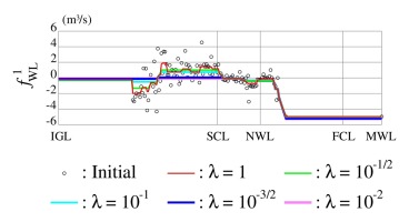
Two five-year subperiods, 2001-2005 and 2007-2011, were extracted from the whole period 2000-2011. Consecutive use of the backfitting algorithm and the TVR identified nominal release policies from the observed release discharges during each of the two subperiods. The increments are chosen as Δt=2π365.25 (rad) and Δh = 0.01 (m). Five cases of the scale parameter λ = 10^–i/2 (i = 0, 1, 2, 3, 4) are considered. The numerical solution of the initial value problem (10) successfully converges to a steady state for each case of λ. Figures 3 and 4 compare the processes of TVR applied to ftime0 for the Main Canal during the two subperiods 2001-2005 and 2007-2011. Figures 5 and 6 compare the processes of TVR applied to fWL0 for the Main Canal during the two subperiods. The value of C⁰, which is equal to the average of all release discharges to the Main Canal, is 12.01 and 15.60 for the subperiods 2001-2005 and 2007-2011, respectively. Then, release discharges to the Main Canal are reconstructed with the nominal release policies identified from the observed data during the two subperiods, as shown in Figures 7 and 8. For example, with λ = 10^–2, Figures 3 and 5 indicate that the values of ftime0 and fWL0 are –8.29 and –0.28, respectively, if the water level is at SCL (EL 8.14) on January 1^st during the subperiod 2001-2005. In that case, the nominal release discharge becomes equal to ftime0 + fWL0 + C⁰ = −8.29 − 0.28 + 12.01 = 3.44 (m³/s). Figures 9-13 show the results similarly computed for the Selinsing Canal as in Figure 3 through Figure 8 for the Main Canal. The value of C¹, which is equal to the average of all release discharges to the Selinsing Canal, is 6.32 and 6.86 for the subperiods 2001-2005 and 2007-2011, respectively.

Fig. 3.

The process of TVR applied to the function of time for the Main Canal during the subperiod 2001-2005.

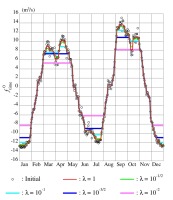
http://www.mhwm.pl/f/fulltexts/154592/MHWM-9-0010-g003_min.jpg

Fig. 4.

The process of TVR applied to the function of time for the Main Canal during the subperiod 2007-2011.

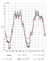
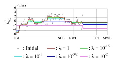
http://www.mhwm.pl/f/fulltexts/154592/MHWM-9-0010-g004_min.jpg

Fig. 5.

The process of TVR applied to the function of WL for the Main Canal during the subperiod 2001-2005.

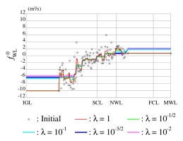
http://www.mhwm.pl/f/fulltexts/154592/MHWM-9-0010-g005_min.jpg

Fig. 6.

The process of TVR applied to the function of WL for the Main Canal during the subperiod 2007-2011.

http://www.mhwm.pl/f/fulltexts/154592/MHWM-9-0010-g006_min.jpg

Fig. 7.

Reconstructed release discharges to the Main Canal with the 2001-2005 policies.

http://www.mhwm.pl/f/fulltexts/154592/MHWM-9-0010-g007_min.jpg

Fig. 8.

Reconstructed release discharges to the Main Canal with the 2007-2011 policies.

http://www.mhwm.pl/f/fulltexts/154592/MHWM-9-0010-g008_min.jpg

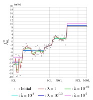
Fig. 9.

The process of TVR applied to the function of time for the Selinsing Canal during the subperiod 2001-2005.

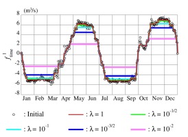
http://www.mhwm.pl/f/fulltexts/154592/MHWM-9-0010-g009_min.jpg

Fig. 10.

The process of TVR applied to the function of time for the Selinsing Canal during the subperiod 2007-2011.

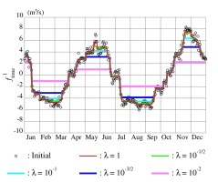
http://www.mhwm.pl/f/fulltexts/154592/MHWM-9-0010-g010_min.jpg

Fig. 11.

The process of TVR applied to the function of WL for the Selinsing Canal during the subperiod 2001-2005.

http://www.mhwm.pl/f/fulltexts/154592/MHWM-9-0010-g011_min.jpg

Fig. 12.

The process of TVR applied to the function of WL for the Selinsing Canal during the subperiod 2007-2011.

http://www.mhwm.pl/f/fulltexts/154592/MHWM-9-0010-g012_min.jpg

Fig. 13.

Reconstructed release discharges to the Selinsing Canal with the 2001-2005 policies.

http://www.mhwm.pl/f/fulltexts/154592/MHWM-9-0010-g013_min.jpg

Fig. 14.

Reconstructed release discharges to the Selinsing Canal with the 2007-2011 policies.

http://www.mhwm.pl/f/fulltexts/154592/MHWM-9-0010-g014_min.jpg

3.2. Choice of the scale parameter

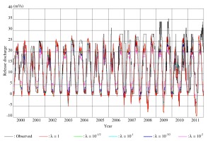
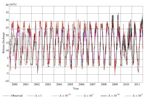
The daily oscillations in f^timek and f^WLk are successfully removed with TVR, while the discrepancy of ftimek and fWLk from them becomes large as the scale parameter λ becomes small. The TV in the reconstructed release discharges tends to decrease for smaller λ. Under the assumption that the release policies are based on the information of t and h_t, the nominal release policies identified by the large-scale parameter λ = 1, are well representative of t and h_t, and thus, considered the most reasonable and realistic.

4. Discussions

4.1. Comparison of the two subperiods

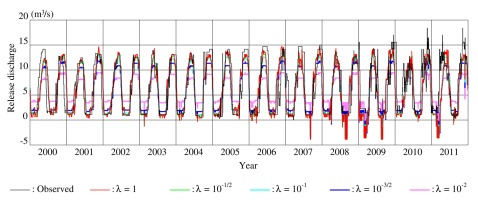
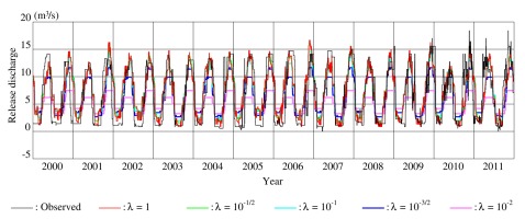
The comparison between the observed and the reconstructed release discharges during the whole period validates the release policies identified from the data during each of the two subperiods. Significant increases in the peaks and the TV of the observed release discharges in both canals can be seen in 2009-2011. Consequently, the reconstructed release discharges with the 2001-2005 policies barely approximate the observed ones in 2009-2011. This indicates that the operator changed the release policies from the subperiod 2001-2005 to the subperiod 2007-2011.

Referring again to Figure 1, the variable hydrological input, which is under the considerable influence of climate change, is considered the primary cause of changes in the release policies controlling the water balance in the reservoir to satisfy the water demand.

The changes in the functions ftimek from the subperiod 2001-2005 to the subperiod 2007-2011 imply the shifts in the actual irrigation demand’s annual patterns, which are susceptible to rapidly developing agronomic practices such as the choice of varieties to adapt the climate change and to meet the increasing food demand. In the Main canal (k = 0), the two peaks of early-March through early-May and early-September through late-October shifted to mid-March through late-May and mid-September through early-December, respectively. In the Selinsing canal (k = 1), the two peaks of early May through late June and late October through late December shifted to mid-April through mid-June and early-November through mid-January, respectively. As a result, May became the most critical month in the subperiod 2007-2011, having the least rainfall and the overwrapping peaks of the release discharges in the two primary irrigation canals. This increasing criticality of May in the water balance of BMR supports the simulation-based prediction by Hamidon et al. (2015). Furthermore, it is noteworthy that the change in rainfall patterns between the two subperiods in the catchment area of BMR is just a symptom of catastrophic regime shifts in the coming decades, according to the recent climatological studies using GCMs (Adib et al. 2020; Adib, Harun 2022; Adib et al. 2022).

The function fWL0 for the Main canal is mostly monotone increasing with respect to h_t, and its increment was amplified from the subperiod 2001-2005 to the subperiod 2007-2011. The function fWL1 for the Selinsing canal was small for the higher water levels during the subperiod 2001-2005 but became not so much during the subperiod 2007-2011. In other words, the two primary irrigation canals became more utilized for draining excess water from BMR in the subperiod 2007-2011 than in the subperiod 2001-2005. This allocation of the two primary irrigation canals for the drainage purpose might be attributed to the small capacity of Kurau River, which cannot manage the discharges required for reasonable flood control.

4.2. Comparison with other approaches

The first key feature of the approach developed here is to decompose a release policy into possibly singular functions of a single independent variable with the additive structure, unlike the standard procedure identifying release policies as quite regular functions of multiple independent variables (Turner et al. 2021). As discussed in the previous subsection, the decomposition of release policies illustrates the two aspects of the irrigation demand’s annual patterns and the hydraulic structures’ functions.

The second key feature is the TVR applied to the decomposed possibly singular functions, breaking through a widespread obsession that policy identification is “to minimize some distance metric between historical releases and modeled ones,” as in Giuliani et al. (2014). This study is the first to succeed in quantitatively treating the indecisive attitude of a reservoir operator as the spurious oscillations to be removed with the TVR. The release policies extracted with the TVRs are the nominal parts. Overgaard (2019) provides mathematical proof to endorse the ROF model in one dimension used in this study for TVR. However, the lack of an established method to choose the best scale parameter λ is a practical limitation of this approach. A follow-up study shall be conducted to validate the λ values with the empirical knowledge of the reservoir operator.

A sophisticated approach is being developed to combine the backfitting algorithm with TVR (Yang, Tan 2018). Nevertheless, our approach, opting for the sequential use of the two procedures, is advantageous because it is not computationally demanding.

5. Conclusions

The consecutive use of the backfitting algorithm and TVR successfully identified the nominal release policies implemented in BMR during each of the two subperiods as the GAMs. The additive structure decomposed the varying parts of the nominal release policies into the two functions. The scale parameter of the TVR controlling the removal of spurious oscillations should be chosen so that the nominal release policies are sensitive to the time and water levels. The results have been utilized to compare the two subperiods, indicating the significant changes in the operator’s release policies. The rapidly developing agronomic practices and the insufficient discharge capacity of the Kurau River receiving the water released from the spillways might be seriously burdening the operation of BMR. We have also addressed the situation in another study (Fadhil 2018), so that the reservoir operator is aware of future hydro-meteorological information, and deducing optimal release policies of BMR based on the SDP theory.

ACKNOWLEDGEMENTS

The authors thank Malaysian authorities, including the Department of Irrigation and Drainage (DID), the Department of Agriculture and Agro-based Industry (DOA), and the National Hydraulic Research Institute of Malaysia (NAHRIM), for the provision of the reservoir management report and spatial and hydro-meteorological data. The Ministry of Higher Education in Iraq and the University of Mosul are acknowledged for providing the scholarship to the first author. This research is funded by Putra Grant No.9406300 from the Universiti Putra Malaysia, Grants-in-Aid for Scientific Research No.16KT0018 and No.19KK0167 from the Japan Society for the Promotion of Science (JSPS), and Bilateral Joint Research Project No. JPJSBP120229922 from JSPS.

REFERENCES (41)

Adib M.N.M., Harun S., 2022, Metalearning approach coupled with CMIP6 multi-GCM for future monthly streamflow forecasting, Journal of Hydrologic Engineering, 27 (6), DOI: 10.1061/(ASCE)HE.1943-5584.0002176.