1. Introduction
India lies at the heart of the classical monsoon region; it is extremely vulnerable to frequent hazards of floods and intense downpours that accompany low-pressure systems (LPS) during the monsoon season (Kale et al. 1994). Such massive floods are critical events, from the standpoint of human impact as well as in terms of geomorphic effectiveness.
The Godavari River has one of the most potent flood regimes in the seasonal tropics (Khandare 2009). Major flood events have been reported for the Godavari River, for instance, in September 1969 (Mujumdar et al. 1970), August 1981 (Pandharinath 1984), August 2006, September 2008 (Khandare 2009) and August 2019. However, information is scant about the causes and effects of such large floods on the Upper Godavari River (UGR). Therefore, the objectives of this paper are to examine the meteorological aspects of large floods, to understand the hydrological characteristics of floods, and to evaluate the geomorphic impacts of floods on the UGR in terms of hydraulic properties and effects.
2. Upper Godavari Basin (UGB): geomorphic setting
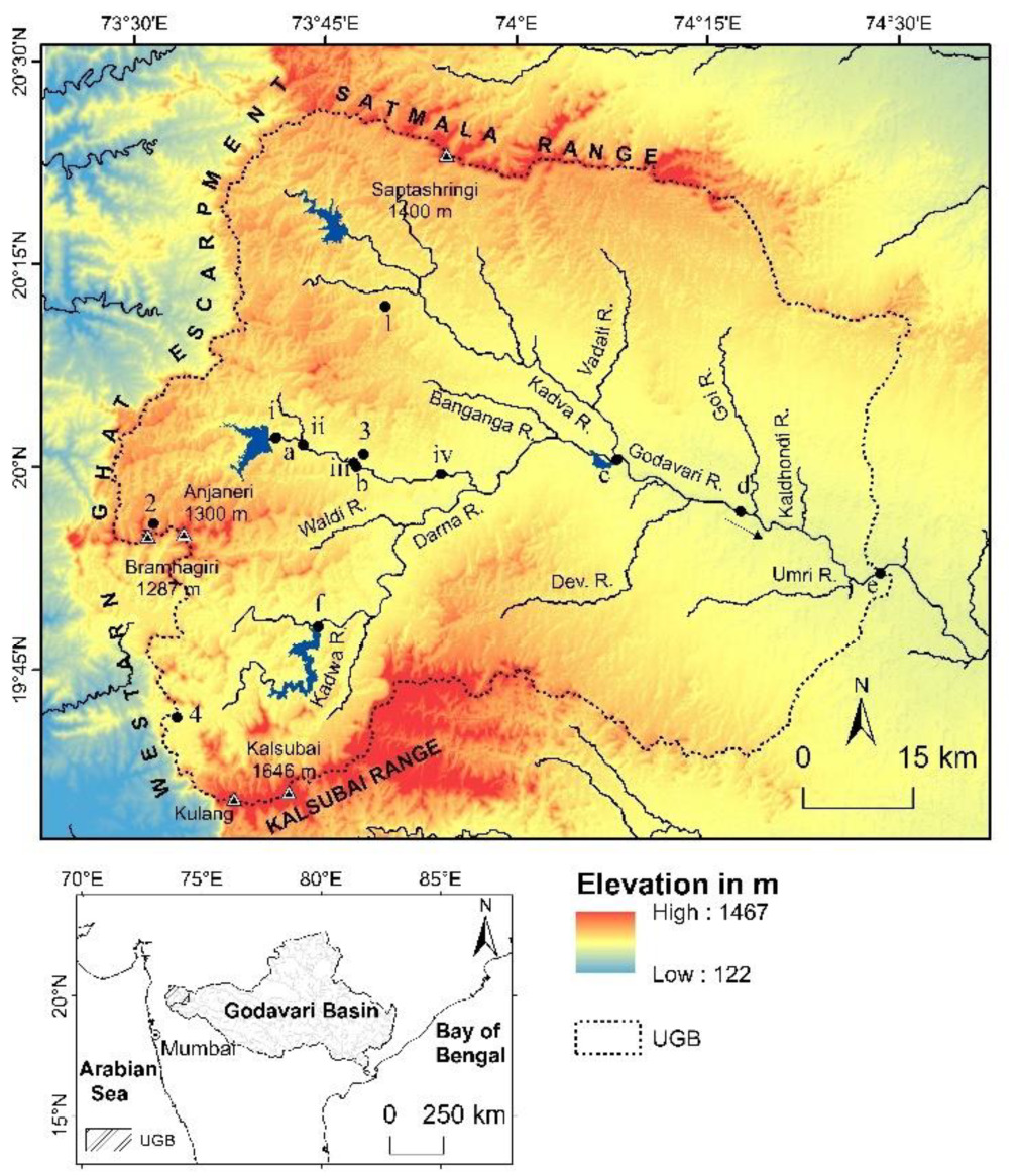
The Godavari River, with 1465 km, is the second longest river in India and the longest among all the rivers in peninsular India. The river rises in the Western Ghat at Bramhagiri near Trimbakeshwar at an elevation of 1287 m in the Nashik District of Maharashtra State (Fig. 1). The river discharges into the Bay of Bengal at Narasapuram in the West Godavari district of the Andhra Pradesh. The total drainage area of the Godavari Basin is 312,813 km2. This study represents an attempt to comprehend the meteorological, hydrological, and geomorphological aspects of large floods of the Upper Godavari River (UGR) in the headwater region (UGB = 5085 km2), i.e., from the river’s source to Kopargaon Tehsil. The UGB is bounded by the Satmala Range in the north, the Western Ghat Escarpment in the west and the Kalsubai Range in the south. Geologically, the region is underlain by Cretaceous-Eocene Deccan Trap basalt; there are no later formations except the older alluvium of the late Pleistocene (Mujumdar et al. 1970) to late Holocene (Kale 2022). The major tributaries of the Upper Godavari River (UGR) are Darna, Dev, and Umri on the right bank, and Kadva, and Goi on the left bank.
3. Data source
Rainfall data from four rain gauge stations in the UGB were employed: Dindori, Trimbakeshwar, Nashik, and Igatpuri, with records ranging from 119 to 143 years (1878 to 2019). The data were collected from the India Meteorological Department (IMD), Pune. Data for tracks of low-pressure systems (LPS) from 1891 to 2019 were derived from the e-atlas obtained from IMD, Chennai. The annual maximum series (AMS) stage data were procured from the Centre Water Commission (CWC), New Delhi, Maharashtra Engineering Research Institute (MERI) and Hydrology Department, Nashik, for five gauging sites on the UGR and one site on its tributary, i.e., the Darna River. The AMS gauge records for the UGR are short and discontinuous (24 to 50 years). The cross-sectional surveys were carried out at four sites to compute parameters of hydraulics and hydrodynamics with respect to high flood levels (HFL).
4. Flood meteorology
Rainfall characteristics in monsoonal regions, particularly the distribution in space and time, are important in terms of flood generation. Consequently, one of the core objectives of this paper is to analyze the meteorological data that are currently available and to pinpoint the characteristics of rainfall that lead to significant flooding on the UGB. The UGR is rainfed, as are its tributaries. The southwest monsoon season’s heavy to extremely severe rainfall is therefore responsible for all flooding on the river. Excessive and widespread rainfall is caused by a range of flood-producing meteorological conditions. These include LPS originating over the Bay of Bengal and terrestrial depressions, along with active to vigorous monsoon activity. In the following section, the features of flood-generating rainfall and allied synoptic situations are depicted. The UGB is located in an environment typical of southwestern monsoonal tropics, with periodic large-magnitude rainfall. The UGB receives 1780 mm of rain on average per year, with monsoon months, i.e., mid-June to early October, accounting for 90% of the total annual rainfall. The rainiest month is July, followed by August; they contribute 37% and 27% of the basin’s total annual rainfall, respectively.
4.1. Interannual rainfall variability and associated floods
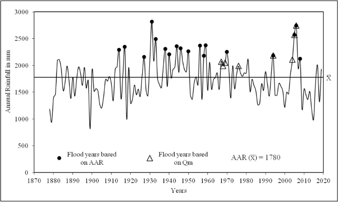
Akin to other monsoon-dominated rivers of India, the UGB also shows significant interannual variation in rainfall and, therefore, flood events. Table 1 lists details of the four stations with long-duration rainfall records (>100 years; between 1878 and 2019). Mean annual rainfall of the UGB ranges from 716 mm at Nashik to 3241 mm at Igatpuri. The low coefficient of variation (CV) (24-33%) of annual rainfall in most parts of the basin demonstrates that interannual variability is not particularly high. The annual rainfall at each site varies greatly (Table 1). For example, the minimum annual rainfall at Nashik was 332 mm in 1984, whereas the maximum annual rainfall at Igatpuri was 6601 mm in 1931.
Table 1.
Annual rainfall characteristics of selected stations in the Upper Godavari Basin (UGB) (from 1878 to 2019). Data source: IMD.
[i] Rmax – maximum rainfall; ASL – above sea level; Rmin – minimum rainfall; AAR – average annual rainfall; σ – standard deviation; Cs – coefficient of skewness; Cv – coefficient of variation. See Fig. 1 for site locations.
The coefficient of skewness (CS) values range from 0.41 to 1.17 and are positive for all of the stations. The Dindori site reveals a relatively high positive CS value. The positive CS values indicate episodes of one or two or a few very wet years during the gauged period, for instance, in 1813 (1376 mm), 1981 (1600 mm), 2019 (1371 mm) and 2017 (1819 mm). Given that CS values have been established based on more than 100 years of data, they are all statistically significant (Viessman et al. 1989).
The interannual variability of rainfall is shown as a time series plot in Figure 2 for the rain gauge sites located in UGB. The figure reveals that previous to 1930, rainfall was commonly below average with low interannual variability. In contrast, in many years between 1930 and 1980, above-average annual rainfall was recorded, with high interannual variability. After 1980, rainfall was frequently below average, with moderate interannual variability. In particular, after the 1930s, interannual variability was marked by an increase in the frequency and magnitude of floods on the UGR. Interestingly, similar results and remarkable interannual variability in the rainfall totals have been reported for some of the westward-flowing rivers of India (Kale 1999; Hire 2000; Patil 2018; Pawar, Hire 2018; Pawar 2019; Patil, Hire 2020; Anwat 2022). The time series plot of interannual variability of rainfall and associated floods shows that almost all of the large flood events in the UGR have occurred when rainfall was above average (Fig. 2). To identify the flood years for the UGR, the annual rainfall and discharge data were analyzed by applying equation 1 (Pant, Kumar 1997) and equation 2.
Ri ≥ AAR + 1σ (1)
where: Ri is the rainfall of year i, AAR is the long-term mean rainfall, and σ is the standard deviation.
Qi ≥ Qm + 1σ (2)
where: Qi is the discharge of year i, and Qm is the mean annual peak discharge.
4.2. Characteristics of the flood-generating low-pressure systems (LPS)
During all months of the year, except February, the Indian subcontinent is subjected to cyclonic disturbances (such as depressions and cyclonic storms) (Dhar et al. 1984). Attributable to the heavy rainfalls associated with these cyclonic disturbances, floods occur in those rivers whose catchments drain the rainstorm area (Dhar et al. 1984). These floods mark the largest recorded peaks in a flood time series (Kale et al. 1994). Flood-producing rainstorms are associated with Bay of Bengal depressions moving westward, general active monsoon conditions over Madhya Pradesh and Gujarat, and terrestrial depressions, according to earlier and more recent studies of the synoptic conditions associated with rainstorms (Abbi, Jain 1971; Ramaswamy 1987; Hire 2000; Patil 2018; Pawar 2019).
An effort has been made to identify and analyze the LPS tracks that caused the highest discharges in the basin to understand the relationship between LPS and floods in the UGB. The e-Atlas software was used to locate the LPS tracks, and ArcGIS 9.3 was applied to analyze them. The buffer zone was delineated at 500 km from the basin margin, and only LPS tracks that passed through the buffer zone were chosen for the investigation (Patil, Hire 2020) (Fig. 3). According to an assessment of the synoptic conditions associated with the flood-generating LPS, several of the LPS in the UGB were the result of Bay depressions and active monsoon conditions over central India. The association of LPS and consequent floods of the UGB were studied by using the AMS data. Streamflow records available for some sites on the UGR and its tributaries indicate that the LPS can have an immense impact. The systems, which comprise lows, depressions, and cyclonic storms (Dhar, Nandargi 1995), cause extreme stream rise, leading to large floods. Table 2 confirms the prevalence of LPS-linked floods in the UGR in August or September, by which time an average of ~42% of the annual rainfall has been received, and soils are completely saturated, further increasing the magnitude of floods.
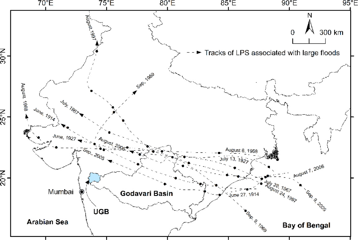
Table 2.
Synoptic conditions associated with major floods on the Upper Godavari River.
In the quadrants to the right of the depression track, the rainfall field is flat. Conversely, large gradients of rainfall subsist in the left quadrants, especially along and west of 80°E. Additionally, the area with the maximum rainfall is in the left front quadrant, 150 km from the center and 50 to 150 km from the depression track (Mooley 1973). The position of the UGB remained in the left front quadrant during transit of the bulk of LPS(s) that traveled WNW or NW (Fig. 3; Table 2), thus resulting in high-magnitude floods. For instance, in 2005 and 2006, LPS caused high flood levels (Qi ≥ Qm + 1σ at Nashik; 633 m3 s-1) on the UGR with 941 and 1034 m3 s-1 discharges, respectively, at the Nashik gauging station. We investigated the relationship between LPS, greatest 24-hr. rainfall, and large floods in the UGB. The highest 24-hr. rainfall at Nashik station was associated with LPS (Table 3). The September 10, 1969, LPS, which transited from the northwest corner of the UGB, is an excellent example of this kind (Fig. 3). The 24-hr. rainfall measured at Nashik station was 183 mm (16% of the total annual rainfall) (Table 3).
Table 3.
Low-pressure systems and highest 24 hr. rainfall at Nashik station. Data source IMD.
5. Flood hydrology
The UGR, similar to other monsoonal rivers of peninsular India, is also subjected to high-magnitude floods at regular intervals. Therefore, it is of paramount importance to know the hydrologic characteristics of floods in terms of magnitude, frequency, and distribution.
5.1. Flood regime characteristics
According to gauge data, mean discharges range between 454 m3 s-1 at Gangapur Dam (GD) and 2178 m3 s-1 at Nandur Madmeshwar Dam (NMD) on the UGR (Fig. 1; Table 4). Historical and modern records show that large floods on the UGR occurred in 1939, 1965 (flood levels marked at Sarkarwada, an old administrative building of the 19th century, Nashik), 1969 (Mujumdar et al. 1970), 1976, 1979, 2004, 2005, 2006, 2008 (Khandare 2009), 2016, and 2019. The highest-ever recorded flood on the UGR at NMD in 1976 was on the order of 9977 m3 s-1. This event, however, was not entirely natural. The unusually high discharge was primarily the result of a sudden release of a large volume of water from the dam. The second largest flood of the UGB occurred on August 10, 2006, with gauged discharge of 8857 m3 s-1 at Kopargaon (Fig. 1). The heaviest 24-hour rainfall, which occurred two days prior to the event, totaled 114 mm, or 9% (Table 3) of the annual rainfall. The other aspects of the UGR’s flood regime are presented in the following section.
Table 4.
Flood flow characteristics of the Upper Godavari River. Data source: CWC.
[i] Qmin – minimum annual peak discharge; Qmax – maximum annual peak discharge; Qm – mean annual peak discharge; A – catchment area. See Fig. 1 for the location of the sites.
5.1.1. Interannual variability in annual peak discharges
The temporal patterns of variability in the annual peak discharges at six sites on the UGB are shown in Figure 4. The graphs reveal high interannual variability in the annual peak discharges and the occurrence of one or two extreme events during the gauge period. A large amount of geomorphic work is accomplished by higher flows in the UGB. Floods that generate discharges several times greater than a river’s mean flows are more likely to result in considerable geomorphic change (Kochel 1988). This effect can be established merely by estimating the Qmax/Qm ratio. The Qmax/Qm ratio for the UGB ranges from 2.39 to 4.89 (Table 4). Consequently, it can be concluded that maximum annual peak discharges (Qmax) are approximately five times larger than average peaks. The significance of higher discharges increases with flow variability (Wolman, Miller 1960). Such high flows are anticipated to have a significant impact on the geomorphic activities in the channel.
Fig. 4.
Interannual variability in annual peak discharges, UGB: (a) Gangapur Dam, (b) Nashik, (c) Nandur Madmeshwar Dam, (d) Chass, (e) Kopargaon, (f) Darna Dam. See Fig. 1 for the location of the sites.
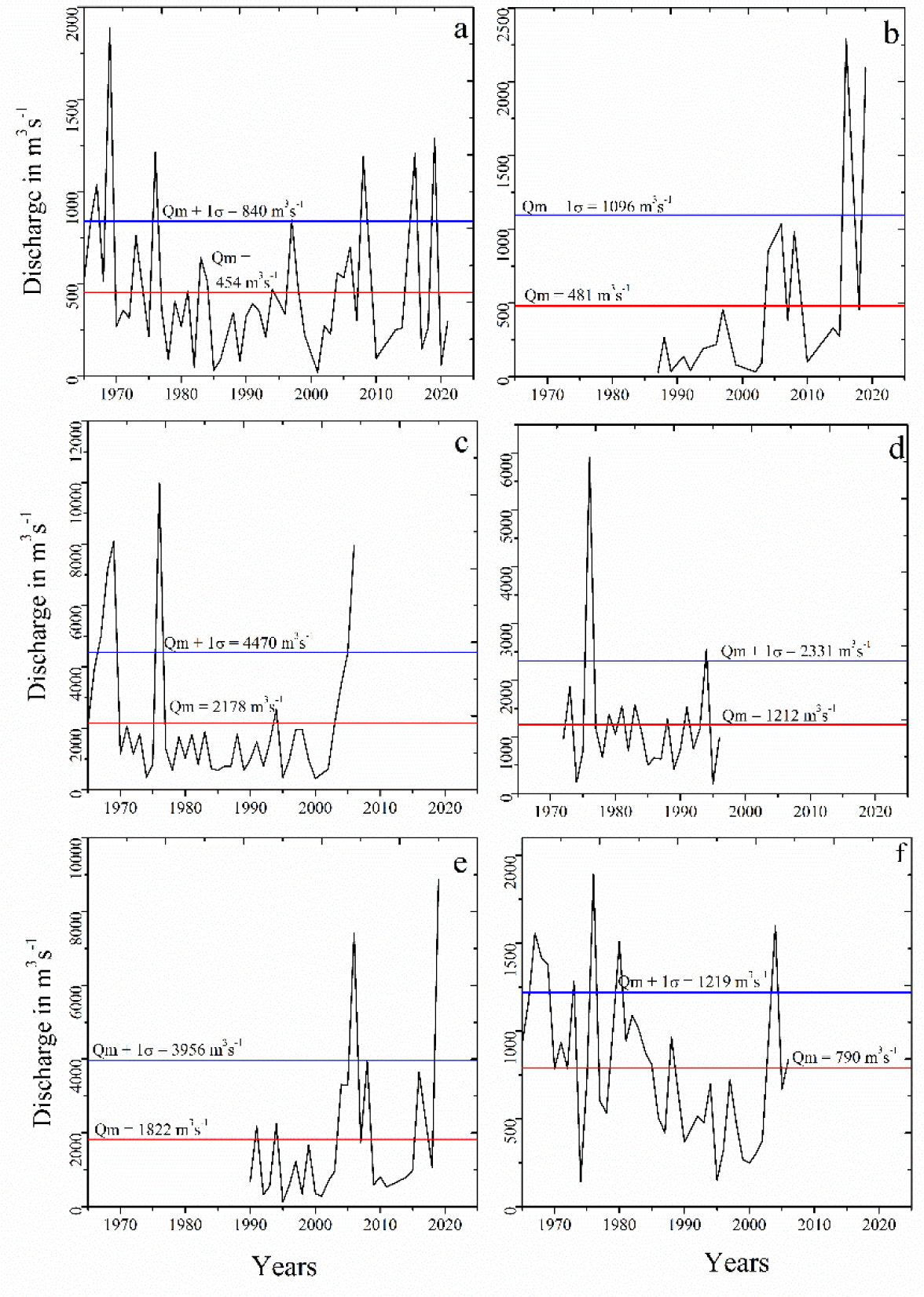
The coefficient of variation (Cv), which measures hydrological variability in annual peak discharges, is another useful indicator. The Cv, which ranges between 0.54 and 1.28 (Table 5), representing the ratio between the standard deviation (σ) and the mean (Qm), suggests moderate to high dispersion. The variability in flood flows may be credited to various hydrological events accountable for producing the floods.
Table 5.
Discharge characteristics of the UGB. Data source: CWC.
[i] Qmax – maximum annual peak discharge; Qm – mean annual peak discharge; SD – standard deviation; Cv – coefficient of variation; Cs – coefficient of skewness. See Fig. 1 for the location of the sites.
A number of researchers have used Beard’s flash flood magnitude index (FFMI) to evaluate the variance in flood frequency as an index of the flashiness of floods (Baker 1977). The FFMI values are calculated using the standard deviation of AMS logarithms, as mentioned below.
where: X is Xm – Qm; Xm – annual maximum event; Qm – mean annual peak discharge; N – number of years of record (X, Xm, and Qm expressed as log10).
The FFMI of the UGB ranges from 0.27 to 0.56, the mean FFMI is 0.4 (Table 6). This FFMI value is greater than the mean for the world, i.e., 0.28 (McMahon et al. 1992; Erskine, Livingstone 1999). The high mean FFMI indicates that UGR floods are slightly more flashy and variable than the average for world rivers. The FFMI further suggests a greater possibility for significant geomorphic changes during large floods.
Table 6.
Flash flood magnitude indices (FFMI) of the Upper Godavari River. Data source: CWC.
[i] See Fig. 1 for the location of the sites.
5.1.2. Skewness
The coefficient of skewness (Cs) is the most common statistical moments employed in investigations of flood geomorphology and flood hydrology. Since the AMS data are not normally distributed, it is vital to find the Cs of the data. The values of Cs for all the stations on the UGR are positive, ranging from 0.65 to 3.34 (Table 5). The Cs values computed for other large rivers in India (Sakthivadivel, Raghupathy 1978; Hire 2000) are similar to the skewness values derived for the UGB. The positive Cs values predict the occurrence of one or two (or a few) very large magnitude flows during the gauge period. However, the characteristic of skewness is of doubtful value when applied to less than 50 years of data (Viessman et al. 1989). Subsequently, some hydrologists have also used the ratio Cs/Cv to further consolidate the degree of skewness (Shaligram, Lele 1978). The Cs/Cv ratio for different UGB discharge-gauging sites ranges from 1.20 to 3.62 (Table 5). The Cs/Cv ratios are often greater than 2.0 for the majority of India’s large rivers (Shaligram, Lele 1978), demonstrating that peak discharge distribution is not extremely skewed.
5.1.3 Unit discharges (Qu)
Unit discharge (Qu) is a crucial indicator of the potential for large floods on a river (Gupta 1988). This ratio divides maximum annual peak discharge (Qmax) by the upstream catchment area (A), giving discharge or water yield per unit drainage area (m3 s-1 km-2). The Qu computed for all the sites on the UGB range from 1.13 to 6.00 m3 s-1 km-2 (Table 7). For the UGB as a whole, the Qu is 3.64 m3 s-1 km-2. These unit discharges fall below the world envelope curve of the unit discharges constructed by Baker (1995). In comparison, the unit discharges of natural extreme floods on large peninsular rivers vary from 0.13 to 0.65 m3 s-1 km-2 (Kale et al. 1997; Hire 2000). In terms of geomorphic changes in the valley and channel, these discharges are likely to be effective (Costa, Connor 1995; Kale et al. 1997).
Table 7.
Unit discharges (Qu) of the Upper Godavari River. Data source: CWC.
[i] A – catchment area; Qmax – maximum annual peak discharge. See Fig. 1 for the location of the sites.
6. Flood geomorphology
Flood geomorphology is concerned with the forms, processes, causes, and effects of floods (Baker 1988). Floods are primarily accountable for sculpting the river channel and the landscape in some hydro-geomorphic environments, for instance, the seasonal tropics (Wohl 1992; Gupta 1995). One of the significant themes in flood geomorphology has been the measurement and evaluation of the geomorphic efficiency of floods of various magnitudes. The geometry of river channels is considered to be a key factor in establishing the geomorphic effect of floods (Kochel 1988). To assess the geomorphic effects of floods, cross-sectional surveys were carried out at four sites (Fig. 5a-d) on the UGR to understand the channel geometry/morphology; hydraulic and hydrodynamic parameters of all the stations for respective high flood levels (HFL) have been computed and analyzed (Table 8).
Fig. 5.
Cross sections, UGR. (a) Dugaon, (b) Someshwar; (c) Sarkarwada; (d) Odha. See Fig. 1 for the location of sites. HFL – High flood level; Red line = 100-year flood line; Blue line = 25-year flood line.
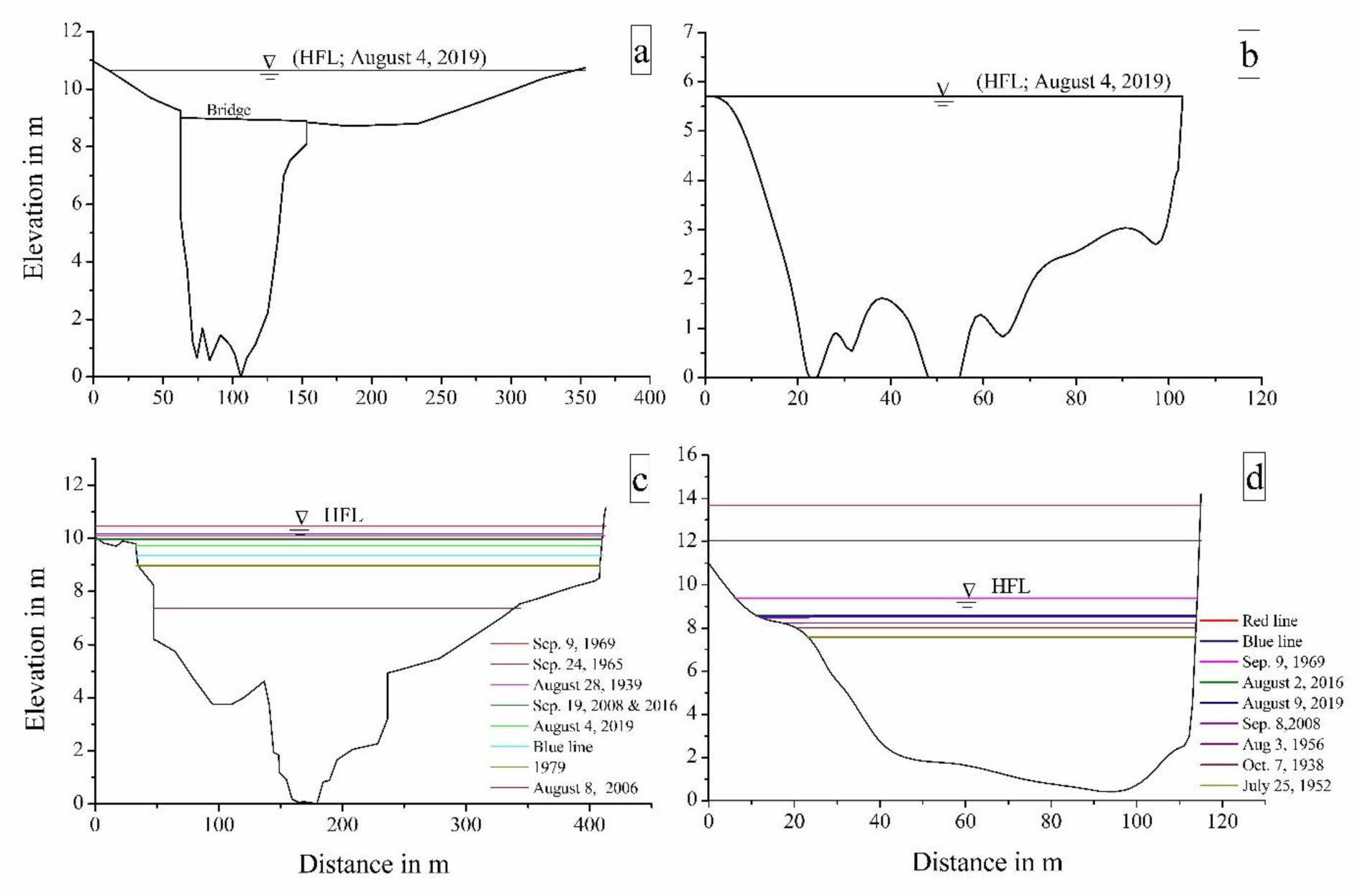
Table 8.
Hydraulic parameters of rare floods on the Upper Godavari River.
The geomorphic efficacy of a flood, which relates to its capacity to affect the shape of the landscape (Wolman, Gerson 1978), is linked to flood power and the degree of turbulence (Baker, Costa 1987; Wohl 1993; Baker, Kale 1998; Kale, Hire 2004, 2007). Therefore, for identified unusual flood events, boundary shear stress (τ), stream power per unit boundary area (ω), Froude number (Fr) and Reynolds number (Re) were computed with the help of the following formulas (Equations 4 to 7) (Leopold et al. 1964; Baker, Costa 1987).
ω = ϒQS/w (4)
τ = γRS (5)
where: ω is unit stream power expressed in watts per square meter (W m-2); γ is the specific weight of clear water (9800 N m-3); Q is discharge in m3 s-1; S is the slope, w is the water surface width in m; τ is the boundary shear stress expressed in Newtons per square meter (N m-2); R is the hydraulic radius or mean depth of water in m. Fr – Froude number;
Critical velocity for inception of cavitation (Vc) is another measure of the erosional power of flows (Equation 8). The Vc in m s-1 is given by Baker (1973) and Baker, Costa (1987).
Vc = 2.6 (10 + D)0.5 (8)
where Vc is the critical velocity for the inception of cavitation in m s-1 and D is flow depth.
The discharges for the unusual floods on the UGR range from 1410 to 6148 m3 s-1 (Table 8). These are large rainfall-runoff floods calculated by indirect methods. From the reconstructed hydraulic data, the stream power per unit area of the UGB ranges from 571 to 5909 W m-2. In comparison, the estimated average unit stream power at a cross-section (alluvial) varies between 322 W m-2 on the Godavari and less than 10 W m-2 on the Brahmaputra (Kale 1998). Estimation of boundary shear stress for large floods by using Equation (5) indicates that the values for UGR range from 192 to 610 N m-2 (Table 8). The estimated values for the Ganga, Yamuna, and Kosi Rivers are 11-25 N m-2, and for the Narmada and Godavari Rivers (as a whole), the shear stress values are >50 N m-2 (Kale, Gupta 2001). Floods generating shear stress of 10 N m-2 can entrain and transport sediments of about 1 cm and can carry sediments finer than 1 mm in suspension (Komar 1988). The high values of shear stress on the UGR reflect the uncommonly high capacity of the river to entrain and transport coarse sediments.
The analysis further indicates that Froude numbers greater than 1 (supercritical flow) have occurred on the UGR at the deep, narrow bedrock reach at Odha (Fig. 1) for all the flow conditions (Table 8). Intense bedrock scouring, resulting from cavitating flow, is also reflected in erosional features such as polished rock surfaces and potholes (Baker et al. 1988; Kale et al. 1993, 1994) at Odha (Fr > 1) and Someshwar sites (Fr ≈ 1). High values of Reynolds numbers signify that the flood discharges could be exceedingly turbulent, and, therefore, capable of a variety of geomorphic actions. The Odha site (Fig. 1) produced the highest Reynolds number (59.12×10⁷) for the September 1969 flood (Table 8), thus, it is probable that this reach experienced very intensive bedrock erosion. The critical velocity for the inception of cavitation (Vc) is a related measure of the erosional power of flows. According to estimates of Vc, no floods have ever exceeded the conditions described by Equation 8 at any of the survey sites on the UGR. However, erosional features, including flute marks, polished rock surfaces, and potholes at various locations at other sites on the UGR, are evidence of severe bedrock scouring by cavitating flow.
The channel bed of the UGR in alluvial reaches is composed of pebbly-cobbly gravel, and of boulders at the Dugaon site (Fig. 1). The sediment-transport equations developed by Williams (1983) were applied to determine the theoretical minimum critical values of bed shear stress (τ), unit stream power (ω), and mean velocity
ω = 0.079 dg1.27 (9)
τ = 0.17 dg (10)
where dg is the intermediate diameter of the grain in mm.
Theoretical estimates indicate that the unit stream power required for moving pebbles (4-64 mm), cobbles (64-256 mm), and a boulder (550 mm) is respectively 16, 90, and 239 W m-2. The corresponding values of boundary shear stress are 11, 44, and 94 N m-2 (Williams 1983). A comparison of these theoretical estimates with the calculated values given in Table 9 specifies that, even though sand and pebbles are moved during all flows, floods on the UGR are capable of transporting cobble-sized sediments, and most of the large floods can move large boulders >550 mm in diameter. For instance, a concrete slab of bridge with i-axis of 810 mm was detached by the August 4, 2019 flood, with an estimated discharge of 2577 m3 s-1 (Table 8) on the UGR at Sarkarwada (Fig. 1). This event produced unusually high values of bed shear stress (272 N m-2), unit stream power (1043 W m-2), and mean velocity (3.83 m s-1) relative to the theoretical threshold estimates (Fig. 6, Table 9).
Fig. 6.
A view of UGR upstream of Sarkarwada (See location in Fig. 1) on 5th August 2019 (a day after the August 2019 flood). Width of flow 128 m and depth of flow 9.71 m (Photograph taken from Holkar/Victoria Bridge, Nashik).
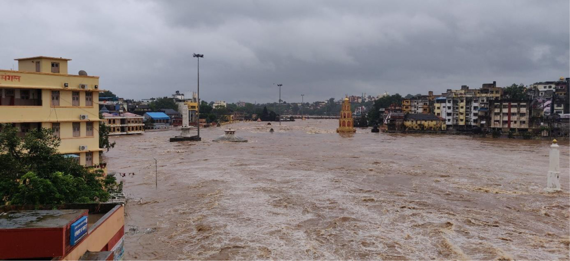
Table 9.
Boulder dimensions at the Dugaon site and the associated theoretical entrainment values.
| Site | Distance from source (km) | I-axis (mm) | τ (N m-2) | ω (W m-2) | W/D ratio | |
|---|---|---|---|---|---|---|
| Dugaon | 30 | 550 | 1.6 | 93.5 | 239 | 16.57 |
| Panchvati(Sarkarwada) | 44 | 810 (Concrete slab) | 5.1 | 405 | 1535 | 39.12 |
Further, the data computed for maximum velocities at Dugaon and Odha range from 3.12 to 9.69 m s-1 (Table 8), respectively. The maximum surface velocities for very large floods are not available. Nevertheless, for the September 1969 flood, the maximum surface velocity was recorded as 2.47 m s-1 at Paithan (Mujumdar et al. 1970), located in an area of gentle channel slope about 215 km downstream from Odha. According to available data, maximum velocities are much higher than the threshold velocities required for the movement of coarse sediment. It is, therefore, certain that large amounts of coarse sediment are moved during large floods, surpassing the total amount of suspended load transported by moderate flows.
7. Conclusions
The southwest summer monsoon (mid-June to early October) dominates the rainfall supply of the UGB by producing about 90% of the annual rainfall. Therefore, the annual flow pattern of the UGB is intimately coupled with the patterns of variation in summer monsoon rainfall. The LPS that originate predominantly over the Bay of Bengal boost the magnitude of rainfall and subsequent floods. Human interference, by releasing large volumes of water from the dams, also underlies changes in flow regimes of the UGB. The study further indicates that the interannual variability of rainfall was associated with increased frequency and magnitude of floods, primarily after the 1930s. High interannual variability persists in the annual peak discharges. The more variable the flow, the more significant the higher discharges become. The maximum annual peak discharges of the UGR are five times higher than average peaks. Therefore, geomorphic activity in the channel is likely to be vital. The slightly flashy and variable nature of floods on the UGR substantiates the possibility of the river experiencing significant geomorphic reworking during large floods. However, unit discharges of the UGR as a whole fall below the world envelope curve of unit discharges constructed by (Baker 1995). The UGR shows high spatial variability in terms of flood hydraulics and hydrodynamics. The higher values for unit stream power and boundary shear stress for rare floods reveal the uncommonly high capacity of the river to erode and transport coarse sediments. The approximate Froude numbers for two sites, as expected, are less than 1, representing that the flows were mainly subcritical. However, Froude numbers >1 for the constricted reach of the bedrock channel at Odha for numerous flood stages revealed that the flows were supercritical. High Reynolds numbers indicate that the flood discharges could be exceedingly turbulent and, therefore, capable of accomplishing a variety of geomorphic activities. According to estimates of the values of critical velocity for the inception of cavitation (Vc), none of the intense floods on the UGR exceeded the conditions required for inception of cavitation. However, erosional features, including flute marks, polished rock surfaces, and potholes at several locations at other sites of the UGR and its tributaries, suggest intense bedrock scouring resulting from cavitating flow conditions. Theoretical estimates of unit stream power, bed shear stress and mean velocity coupled with transported large boulders indicate that the floods on the UGR are competent to move large boulders. The effectiveness of large-magnitude flood events is also evident from the presence of deep, narrow gorges, scablands, polished rock surfaces, inner channels, and waterfalls at several locations on the UGR.