1. Introduction
The design and construction of water systems, as well as water resource management, requires in-depth knowledge of different flood events for different return periods (Tao et al. 2002). The faulty design of engineering structures will have a serious economic impact due to structural damage. Over-designing or under-designing of a hydraulic structure may result in the waste of natural resources or may compromise the structural safety (Reich 1961, 1963). Developing such designs becomes more challenging because of the impact of greenhouse gases, which are changing the hydrological cycle, precipitation patterns, and temperature regimes. Increasing temperatures are altering the physical characteristics of catchments by melting snow and glaciers (Singh et al. 2018). Researchers are thus challenged to devote more effort to analyzing discharges in the water sources for planning and management.
Adequate discharge data are required for the study, analysis, and quantification of various parameters, including design flood. Hydrological stations are not established in all rivers due to economic and geographical limitations, and hence hydrological analysis in such areas is complicated. The availability of discharge data in Nepal is limited. Rivers that descend from hilly areas of Nepal carry large amounts of sediments, so for the un-gauged rivers, the design of hydraulic structures such as weirs, canals, sluice gates, and dams become more complex (Sapkota et al. 2016). Therefore, the main objective of this study is to estimate flood discharges at specific place in ungauged river basins for various return periods, compare estimates and determine the best fit.
The discharge used for the design of a hydraulic structure is called the “design flood”. Designing hydraulic structures for the maximum possible flood for a catchment is very costly. Engineering structures, whose failure may lead to huge loss of lives and properties, are generally designed for floods of large return periods (Izinyon et al. 2011). Design flood estimation is essential for the design of hydraulic structures, flood management and insurance studies, development, and planning. (Rahman et al. 2013).
Hydrologic events have random probability distributions for which statistical analysis can be performed, but precise predictions might not be achieved. Flood frequency analysis is used to estimate design floods for sites along a river that uses observed flow discharge data to calculate statistical information, which is utilized to construct frequency distributions. There is no specific rule for the length of data required for the frequency analysis. Parameter estimation techniques in flood frequency analysis include the graphical method, frequency factor method, method of moments, and method of probability-weighted moments and L-moments (Ojha et al. 2008). Flood frequency estimation is a challenging task for a researcher and has been associated with confusion and controversies (Bobee et al. 1993). Flood frequency analysis helps to predict future flows of different magnitudes and provides reliable predictions in regions of similar climatic conditions. A wide range of research has been conducted to predict the suitable probability distribution functions for annual maximum flood events. Some of the commonly used probability distribution functions include general extreme value, log-normal, normal, Gumbel, Weibull 3P and log Pearson methods. For analysis of the short-term annual maximum discharge, there is no strict rule for using a particular distribution function (Alam et al. 2016).
The bed slope is steep in the mountainous rivers where water flows rapidly, and it is necessary to predict floods for various return periods to design hydraulic structures. Hydropower generation is most common in these rivers. Therefore, designing hydraulic structures like levees, guide walls, dams, intakes, weirs, and barrages need estimates of 10, 20, 50, 100, 200 etc. years return period floods to reduce the risk. Return period flood predictions differ based on the hydrologic distributions selected.
2. Study area
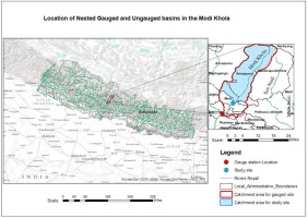
Modi Khola is a major tributary of the Kali Gandaki River, which originates from the Annapurna Conservation area of Nepal. The study basin (Fig. 1) has an area of 510 square kilometers. The location selected for study is at 28.273 N and 83.744 E, in the Parbat district. Climate varies from warm temperate to alpine (Rijal 2007), and most of the precipitation occurs during monsoon season (June, July, August, and September). Quartzite, phyllitic slate, schist, and gneiss were found during a site visit. The sediment yield in the river is high because of the steep gradient, erosion of riverbanks, and fragile geological conditions in the upper part of the river basin. Modi Khola carries sediments ranging from sand to huge boulders during the monsoon, eroded from the banks and transported into it by its tributaries. Many hydropower projects are in operation or under construction; there are also new projects proposed for this river.
3. Methodology
3.1. Data collection
Daily discharge data used in this study are collected from the Department of Hydrology and Meteorology, Government of Nepal, from 1976 to 2010, except data from 1980 to 1987 were not available. The flow data available were point discharge data measured once a day at Nayapul near Jhapre Bagar.
3.2. Analysis
The oldest and most common technique to estimate the daily flow of an ungauged catchment with the use of a reference catchment is the drainage area ratio method (Archfield, Vogel 2010; Gianfagna et al. 2015). Our study catchment is part of a gauged catchment therefore we used the drainage area ratio method for the nested watersheds.
where Q1 and A1 are discharge and area for the gauged catchment, and Q2 and A2 are discharge and area for the ungauged catchment.
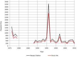
Annual maximum discharge data were obtained from the dataset for each year by selecting the largest daily flood from that particular year. For hydrological analysis, these data were transferred to the selected outlet point of the study basin by the drainage area ratio method; the data are plotted in Figure 2.
For flood frequency analysis using peaks above threshold, identifying such large floods from years of daily data is difficult. We simplified this job by taking the largest flood in a monthly interval from the chunk of daily discharge data. This data series cutoff value was set equal to the smallest discharge from the annual maxima series at Nayapul Station. The selected 61 discharge data points were then transferred to the study basin using the drainage area ratio method. For partial flood frequency analysis, we calculated the average return interval (ARI) from these selected floods. The average number of occurrences of peak flood events (k) is equal to 61events divided by 27 years, i.e. 2.26 events per year. After adjusting ARI to k times ARI, the flood values were predicted based on the adjusted ARI values from various distribution functions.
To select the best fit probability distribution, first of all, alternative probability distribution models need to be analyzed. Continuous probability distributions used in the hydrology sector, including generalized extreme value, Gumbel maximum, log Pearson type III, log Normal (3P), normal, and Weibull 3P were fitted to the processed flood data. The regional empirical methods Hydest and Modified Hydest were used for predicting discharges for different return periods.
3.3. Theoretical description
3.3.1. WECS/DHM method (Hydest Method)
The WECS/DHM method was developed by the Water and Energy Commission Secretariat, Department of Hydrology and Meteorology (WECS/DHM) of Nepal. This method is generally used to determine the hydro-logical features of an ungauged basin for the pre-feasibility study of hydro-electric projects in Nepal. For this purpose, the whole country is considered as a single hydrological region, and the method is suitable for any basin with area ≥100 km2. Hydest is available in the form of an Excel file, which requires input for total catchment area, area of catchment below 5,000 m elevation, area of catchment below 3,000 m elevation, and monsoon wetness index.
Instantaneous peak flood discharges for return periods of 2 and 100 years are:
Peak flood discharge for different return periods:
where: Q2 – two-year instantaneous flood in m3/s; Q100 – 100-year instantaneous flood in m3/s; QT – T-year instantaneous flood in m3/s; Abelow 3000m – basin area below 3000 m elevation in km2; σ is a parameter; S is a standard normal variate whose value depends on return periods (Table 1).
3.3.2. Modified Hydest
This method is the updated version of WECS/DHM method in which one more parameter, basin average elevation, is also taken into consideration.
For 2- and 100-year return periods, flood discharges are given by:
Peak flood discharge for other return periods (T):
The relationship between T and S is shown in Table 1; where: Q2 – two-year instantaneous flood in m3/s; Q100 – 100-year instantaneous flood in m3/s; QT – T year instantaneous flood in m3/s; Abelow 3000m – basin area below 3000 m elevation in km2; σ is a parameter; S is a standard normal variate whose value depends on return periods.
3.3.3. Goodness of fit tests
The goodness of fit technique is a method of examining how a sample of data aligns with a given distribution as its population (Wickramaarachchi 2016). The data were fitted in the EasyFit software (https://easyfit.soft32.com/) to check fits for distributions common in hydrology, and then floods for selected return periods were predicted.
4. Results and discussions
The discharge data were obtained for 27 years, and maximum annual discharge data were calculated from maximum daily discharge values. Sixty-one peaks above threshold flood over a period of 27 years were taken to predict floods for various return periods. There is no particular rule for establishing the trim level for partial frequency analysis, so we took the lowest annual maximum value as our trim level, and floods greater or equal to that value were fed into probabilistic distribution models. The data were evaluated with the probability distribution functions mentioned above to determine the flood discharges for return periods of 2, 10, 20, 50, 100, and 200 years. Comparisons of the different frequency analysis methods and empirical methods are shown in Tables 2, 3, and 4.
Table 2.
Floods [m3/s] of different return periods using different methods for annual maxima (GEV = generalized extreme value, LP 3 = log Pearson, Type III, LN = log Normal, 3P = Three Parameter.
Table 3.
Floods [m3/s] of different return periods using different methods for peaks above threshold.
Table 4.
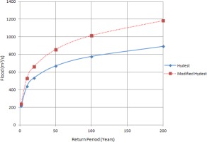
Floods [m3/s] of different return periods using empirical methods.
| Empirical Methods | ||
|---|---|---|
| Return period T (years) | Hydest | Modified Hydest |
| 2 | 216 | 240 |
| 10 | 438 | 531 |
| 20 | 535 | 665 |
| 50 | 670 | 858 |
| 100 | 778 | 1016 |
| 200 | 892 | 1186 |
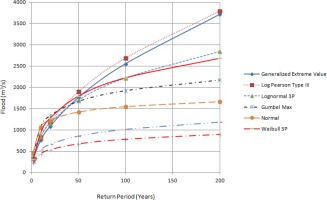
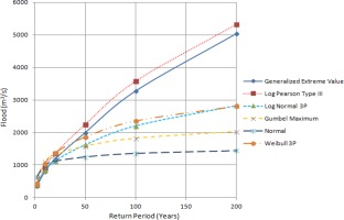
Estimated floods are presented in Tables 2, 3, and 4 for comparative analysis. Figures 3a, 3b, and 3c also provide information about floods of different return periods using various methods. It has been found that the estimated flood values from different methods diverge for higher return periods. The best fits of distribution functions are shown by ranking in Tables 5 and 6. When designing hydraulic structures for a river like Modi Khola, the choice of distribution to estimate the flood for different return periods should be based on the fit of the distribution to the discharge data. From Table 4, we found that Hydest and Modified Hydest estimated smaller floods than other frequency analysis methods.
Table 5.
Fitness of hydrologic distributions for annual maxima.
Table 6.
Fitness of hydrologic distributions for peaks above threshold.
To fit the probability distribution functions with the flood data at a certain significance level (α) × 100%, the test statistics and critical values were analyzed. The test statistics for different kinds of tests: Kolmogorov Smirnov (K-S), Anderson Darling (A-D), and chi-squared (χ2) should be less than the critical value corresponding to significance level α.
The following tables give the details of the probabilistic analysis carried out for annual maximum floods and peaks above threshold.
Each distribution was assigned a rank, the first rank indicating the best fitting distribution, and the last indicating the worst fitting among the distributions used for comparison. The N/A value indicates that the distribution is not applicable for the given data at the 5% significance level and hence rejected. From Tables 5 and 6, generalized extreme value and log Normal (3P) functions are accepted at a 95% confidence interval.
5. Conclusion
The frequency analysis of annual maximum and peak discharges above threshold for identifying the best fit probability distribution was performed using normal, Gumbel maximum, log Pearson type III, log Normal (3P), generalized extreme value, Hydest, Modified Hydest and Weibull 3P distributions. Most of the research on flood flow estimations has been conducted at gauged locations, with very little research for ungauged locations. Estimating flood discharges at different locations in an ungauged catchment requires a hydrologically similar reference catchment, the choice of which is a challenge.
For our study basin, based on K-S, A-D and χ2 tests, we found that GEV and LN (3P) are well fitted compared to other hydrological distributions. Selection of the suitable distribution also depends upon financial considerations as well as risk optimization. Designing hydraulic structures based on the design floods from the GEV distribution may not be cost-effective because of the large predicted flood values for larger return periods, so the LN (3P) can be suggested as an alternative. This study indicates that at least GEV and LN (3P) distributions are better suited for flood frequency analysis of an ungauged basin where the geographical and hydrological features are similar to that of the study basin.
Nevertheless, the limited data available for both spatial and temporal resolution for the gauged basin should be acknowledged, and the hydrological similarities between the catchments should be carefully assessed; these characteristics can vary drastically from one place to another. A cross-check of transferred data should be done where another similar catchment is available to enhance the credibility of the data while selecting the appropriate method. Hydest and Modified Hydest are commonly used in Nepal for preliminary assessment of the hydrology of ungauged basins.
The methodology we used in this study can be adopted to study the hydrology of an ungauged site in the basin where the hydrological and meteorological stations are very sparse. Because of epistemic as well as alea-tory uncertainties, we cannot exactly quantify the hydrological characteristics of even the gauged river basins. Moreover, for ungauged basins, epistemic uncertainty is significantly high. Therefore, we should be skeptical about our probabilistic analysis while selecting the appropriate distributions, and thus a comparative analysis of hydrological distributions for different tests is recommended. Moreover, choosing a probability distribution function does not depend only on its goodness of fit but also on the optimization of hydraulic structures based on safety and cost. Therefore, this study helps in estimating return floods for various return years in ungauged basins and in selecting design flood for engineering structures, in developing hydrology models, agriculture, flood management, river training works, and environmental studies.

