1. Introduction
In Antarctica, the near-surface wind (NSW) regime is no less important than changes in the air temperature; both of these characteristics are used to analyze the state of the global and regional climate (Parish, Cassano 2001; Ramesh, Soni 2018). NSW in the coastal zone and over continental Antarctica is partially related to atmospheric circulation and its intensity (Tymofeyev et al. 2017; de Brito Neto et al. 2022). Therefore, changes in the NSW regime reflect changes in the climate system over all of Antarctica. Spence et al. (2014), Hazel (2019), and Alkama et al. (2020) showed that changes in the NSW regime around Antarctica affect the continent’s ice shelves. Thus, in the NSW regime, there is a decrease in the magnitude of easterly and southerly wind components and an increase in the magnitude of the westerly wind component. Because the westerly winds, generally of marine origin, are warmer, there is greater heat transfer to the floating glaciers of Antarctica and, accordingly, melting of the ice sheets. The latter effect contributes to global sea level rise. Some studies assess the potential of Antarctic flows to generate wind energy (Yu et al. 2020; Wang et al. 2023), and it has been shown that the strongest winds on Earth close to sea level are formed over Antarctica at coastal sites in Adélie Land (Parish 1988; Turner et al. 2009). However, the low air temperatures make working there difficult for man and machine alike (Yu et al. 2020).
Usually, in Antarctica, changes and trends in NSW are studied through observations from meteorological stations and through reanalysis (Tymofeyev et al. 2017; Dong et al. 2020). Although observations yield reliable information about the characteristics of the wind in specific places in Antarctica, the data contain gaps and incorrect values. The number of gaps, in relation to the total length of the data series, are, however, generally few. For example, at the Vernadsky Station, missing data are approximately 0.07% of the total (Tymofeyev et al. 2017). Gaps in the data record may be caused by interruptions in observations due to the replacement, repair, and adjustment of equipment. Incorrect values may be related to both human errors in recording and the difficulties of conducting instrumental observations in harsh weather conditions. In addition, research stations are predominately located near the Antarctic coasts, which results in fewer observational data records for studying the central part of the continent. Reanalysis of data makes it possible to obtain a spatial distribution of the NSW, however, mitigating certain limitations of the observational data. While this approach generalizes and simplifies the characteristics of the NSW, it does allow for obtaining its general tendencies (Turner et al. 2009).
At the Vernadsky Station, the NSW regime is shaped by regional features such as the local foehn winds, which are generated in the mountains of the Antarctic Peninsula (King, Turner 1997). Many researchers use the observational data from this station to investigate the changes, variability, and tendencies of the NSW regime (van Lipzig et al. 2004; Turner et al. 2009; Tymofeyev et al. 2017; Dong et al. 2020; Andres-Martin et al. 2024). For example, van Lipzig et al. (2004) modeled the NSW regime over the Antarctic Peninsula, including data from observations from the Vernadsky Station. Turner et al. (2009) reported that since the 1950s, one of the greatest statistically significant increases in the NSW speed has been in the area of the Vernadsky Station. Tymofeyev et al. (2017) reported that, according to the data from the Vernadsky Station, an increase in the NSW speed is seen under conditions of increased air temperature, which is a manifestation of climate change in the study region. This phenomenon reflects changes in atmospheric circulation, primarily the strengthening of the westerly wind and increase of cyclogenesis in the Antarctic. Statistical inhomogeneity in the wind speed series was revealed. Dong et al. (2020) reported that six recent global reanalysis products show positive trends in the annual and summer wind speeds for the 1980-2018 period, which are linked with positive polarity of the southern annular mode. It should be noted that observational data from the Vernadsky Station were also used as input to the reanalysis. Andres-Martin et al. (2024) reported that the observed annual trends in the NSW speed exhibit a generally positive trend, marked by a strong seasonal variability at the northern Antarctic Peninsula.
The Vernadsky Station NSW speed data require careful assessment of homogeneity and stationarity. Such analysis is also needed in view of climatic changes, which can cause violations of the homogeneity and stationarity of observational series. In previous studies (Tymofeyev et al. 2017; Andres-Martin et al. 2024), the NSW homogeneity, stationarity, and tendencies at the Vernadsky Station were analyzed exclusively by statistical tests. Kundzewicz and Robson (2000; 2004) recommended applying more graphical analysis to confirm the results of evaluating the tendencies of time series by standard statistical tests. Graphical analysis is especially important when statistical analyses do not have unambiguous interpretations or when only one statistical test (or several statistical tests with the same properties) is used (Robson 2002). So, for more reliable results, a complex approach using various tests and methods is recommended (Kundzewicz, Robson 2004; Gorbachova et al. 2022).
A significant amount of research is devoted to statistical analysis of time series. Much scientific interest was sparked by the monograph of Box and Jenkins (1970), in which the methodological foundations of time series analysis in various fields, such as economics, natural sciences, etc., were developed. The most widespread methods for assessing the homogeneity and stationarity of an observational series are various parametric and non-parametric statistical criteria (tests) described and recommended by WMO guidelines (WMO 1990; 2018). Criteria such as the Alexandersson, Terry, Buishand, Pettitt, Spearman, von Neumann, Wald-Wolfowitz, and Mann-Kendall tests are the most widely used.
Graphic analysis of the homogeneity and stationarity evaluation of observation series is based on various graphs, such as correlation (x/y plot), histogram, mass curve, double mass curve, residual mass curve, and chronological graph. Among these, mass curve analysis, double mass analysis, and residual mass curve are the most widely used. Klemeš (1987) and Gorbachova (2016) reported that at the end of the 19th and during the 20th century, these methods were developed by W. Rippl, A. Schoklitch, J. Novotny, C. Merriam, M. Kohler, L. Weiss and W. Wilson, J. Searcy and C. Hardison, and K. Ehlert. The methods of the mass curve and residual mass curve were developed by Rippl (1883). Subsequently, Schoklitsch (1923) and Novotny (1925) proposed to calculate the residual mass curve of the mean flow value (Klemeš 1987). In 1937, Merriam invented a double mass curve for flow analysis, combining precipitation and river flow information. Kohler (1949) proposed using the slope coefficient of the double mass curve to correct violations of the homogeneity of a series of precipitation observations. Weiss and Wilson (1953) investigated the estimation of significance of change in the double mass curve slope. Searcy and Hardison (1960) developed a fundamental method for analysis of time series based on the use of a double mass curve and a residual mass curve for homogeneity analyses of observation series of precipitation, hydrologic flows, and sediment flow. Ehlert (1972) presented a modified version of the double residual mass curve in which the relative accumulation of deviations derives from the mean of two observation series, used to homogenize the precipitation observation series. In these investigations, methodological recommendations for applying each approach separately and for solving a separate task were developed. More recent approaches to assessing the homogeneity and stationarity of observation series using graphical methods have been developed by Gorbachova (2014; 2016), and applied to analyses of hydrometeorological observation series (Gorbachova et al. 2018; 2022; Romanova et al. 2019; Zabolotnia et al. 2019; 2022; Khrystiuk, Gorbachova 2023).
The objective of this paper is to investigate the homogeneity, stationarity, and tendencies of NSW speed at the Vernadsky Station based on a combined analytical approach, one consisting of the use of several statistical and graphical methods. These methods are described in Section 2, while in Section 3 they are applied in analyses of the data.
2. Study area, data, and methods
2.1. Study area
Until 1996, the Vernadsky Station was the British Faraday station. On February 6, 1996, the British flag was solemnly taken down, and the flag of Ukraine was raised. The Vernadsky Station is located off the western coast of the Antarctic Peninsula on Galindez Island, Argentine Islands Archipelago (Fig. 1), at coordinates 65.25°S, 64.27°W. The climate is marine subarctic, dominated by large-scale circumpolar circulation in the atmosphere and ocean (King, Turner 1997).
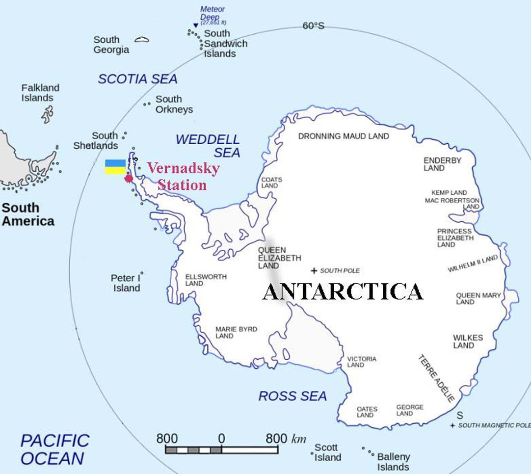
The mountains of the Antarctic Peninsula and the meridional orientation of its coastline are the chief influences on NSW and air temperature regimes in the area of the Vernadsky Station (Turner et al. 2009). As a result, these regimes are specific to the locality, a matter discussed in detail by Gorbachova et al. (2022), Khrystiuk et al. (2023), and Shpyg et al. (2024).
2.2. Data
In this study of the period 1955-2022 at the Vernadsky Station, the NSW speed data (10 m above ground) for eight measurements per day (0, 3, 6, 9, 12, 15, 18, 21 UTC) were provided by the state institution National Antarctic Scientific Center, Ukraine (NASC). Over the life of the Vernadsky Station, various instruments and complexes have been used to measure NSW speed. From 1955 to 1966 a Munro Mk. 1 indicator was used to measure wind speed, followed from 1967 to January 1976 by a Munro Mk. 1B indicator.
Since February 1976, a Munro Mk. 4A indicator has been installed at the station, and in March 1980 it was transferred to a new weather mast. During January 10-24, 1984, an automatic meteorological station SCAWS (Synoptic and Climatological Automatic Weather Station) was installed and tested, and on January 1, 1986, it began to be used in operational mode; that is, this date must be considered the date of the device update. In December 1990, the MAWS (Modular Automatic Weather Station) automatic weather station was installed and on April 1, 1992 began to be used in operational mode. Since February 20, 2011, a Ukrainian-made Mobile Meteorological Complex (MMC), “Troposphere” (Mobile AWS “Troposphere”), became the main measuring complex at Vernadsky Station. In February 2019, MAWS was dismantled, and a Vaisala AWS-310 automatic weather station was installed, which began working in test mode. Measurements from MMC “Troposphere” continue to be sent to the data exchange system of the World Meteorological Organization. On April 1, 2020, the official transition to the Vaisala AWS-310 automatic weather station was made, and it became the main source of meteorological data for the international exchange system (i.e., formation of WMO SYNOP and CLIMAT summaries). Currently, MMC “Troposphere” works as a reserve. So, the Vernadsky and record of NSW speed contains gaps incorrect values resulting from frequent replacement of equipment.
Therefore, the Vernadsky NSW speed data were checked for missing values and gross errors. This process involved two stages: a semantic check and a review of the data based on parameters of the meteorological values. The semantic check was done to identify cases when year, month, date, time, and values of NSW speed were missing using the British Antarctic Survey database; it included searching for missing measurement record identifiers (e.g., values of –99.9). Furthermore, a more detailed analysis of the series of observations revealed the presence of several types of errors, with examples as follows:
− Explicit errors in recording the meteorological value. These are revealed when a value goes beyond the data range obtained over the entire period of observation, or when a value is significantly greater than the nearest two measurements.
− Implicit (hidden) errors. These are identified when the value of the meteorological quantity seems correct by itself, but the value appears erroneous in the context of another additional meteorological quantity or quantities. For example, a wind speed value is zero, but a wind direction value is reported (i.e., has values from 1° to 360°).
2.3. Methodology
The homogeneity, stationarity, and trends of the NSW speed series at the Vernadsky Station were evaluated with a combined approach comprising five statistical and three graphical methods. Statistical homogeneity means that the statistical properties of any one part of an overall dataset are the same as any other part (WMO 1990). Homogeneity was tested by two parametric (standard normal Alexandersson, Buishand) and two non-parametric (Pettitt, von Neumann relation) methods. Stationarity of the observation series means that its statistical characteristics do not change over time. In stationary time series, there is no trend in the mean or variance over time (WMO 1990). In this study, establishing the trend equation for the time series and correlation coefficients between variables were determined by the Pearson method. The statistical significance of the trend was evaluated using the non-parametric Mann-Kendall test.
The series was processed using RStudio Software 1.4.1717 with the following functions (R Core Team 2017):
− pettitt.test – Pettitt test;
− br.test – Buishand test;
− snh.test – standard normal Alexandersson test;
− VonNeumannTest – von Neumann relation;
− MannKendall – Mann-Kendall test;
− gml – construction of a linear trend;
− cor.test – determination of the correlation coefficient by the Pearson method.
Graphical methods make it possible to trace trends over time and identify periods of change, if any, to analyze cyclic fluctuations and their characteristics (e.g., phases of increase and decrease, their duration, synchronicity, and phasing). Three graphical methods were used in this research: mass curve, residual mass curve, and chronological graph. A mass curve is a graph of cumulative values of hydrometeorological characteristics, which, under constant conditions, is a straight line with a slope, relative to the abscissa axis, that is constant over time. The deviation of the hydrometeorological characteristic from a straight line on the graph is an indicator of change that implies change in the controlling factors, e.g., a change in the climate regime (Gorbachova 2014; Gorbachova et al. 2022). Short- and long-term cyclical fluctuations can be investigated by the residual mass curve. The residual mass curve is a graph of successively accumulated deviations of a hydrometeorological value from its initial value, for example, an arithmetic mean, depending on time or dates (Gorbachova et al. 2022). The chronological graph allows one to trace the changes and fluctuations of a hydrometeorological characteristic over time.
3. Results
3.1 Primary analysis of observational data
For the period 1955-2022 at Vernadsky Station, the observational data for NSW speed contains 198,696 points, of which 27,377 (almost 14% of the total number) have gaps and incorrect values (Fig. 2). Gross mechanical errors and significant outliers in the observation series were removed.
Fig. 2.
The number of gaps and incorrect values (missing records) of observation series of the near-surface wind speed in the area of the Vernadsky Station in 1955-2022.
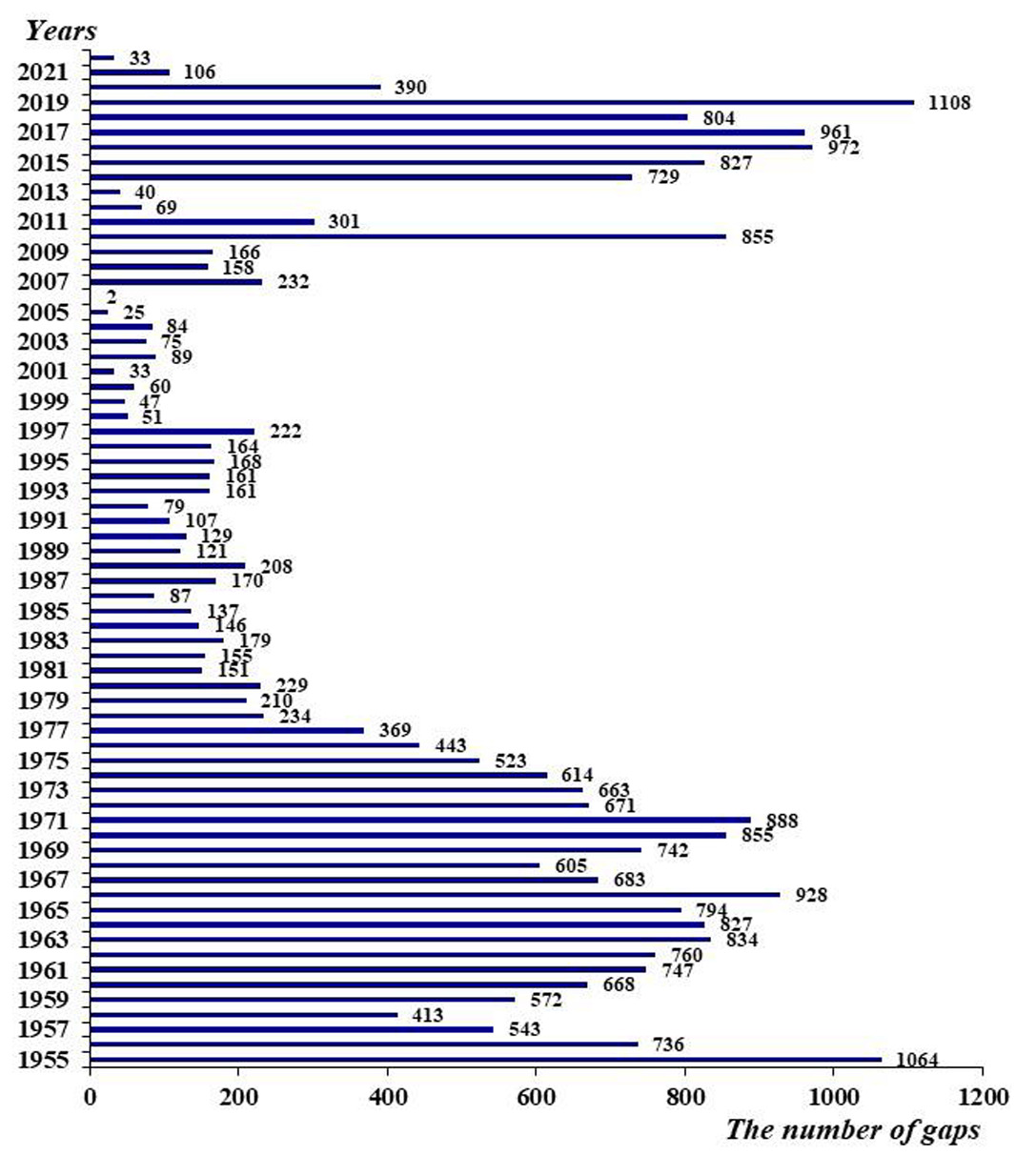
Most of the data that were considered erroneous and excluded from the research series in the period of 2014-2019 related to incorrect operation of the software, which occurred at low wind speeds and when wind changed direction through the 360° mark. The annual average number of observations is 2966. The largest number of gaps and incorrect values in the observations (1064) occurred in 1955, and the smallest number occurred in 2006 (2) (Fig. 2). There was also a significant number of gaps and incorrect values in the observations in 2019 (1108).
Based on eight measurements per day (viz., measurements every three hours), daily averages and mean monthly and mean annual values of the NSW speed were calculated. Mean monthly values of the NSW speed were not calculated for those months in which the number of missing records in the observations was 33% or more of the total number of records, where there were no observations for three consecutive days or more, or where there were 10 or more missing records in the observations at a given observation time (i.e., 0, 3, 6, 9, 12, 5, 18, or 21 UTC). Mean annual values of the NSW speed were not calculated for those years in which mean monthly values were not determined for four months of the year or if mean monthly values were not determined for two or more consecutive months in the year.
After data quality control, it turned out that even though the total duration of observation was 68 years, the mean duration of all of the records was only 49 years. The longest record of NSW speed has observations for 58 years (September), and the shortest record for 39 years (mean annual NSW speed) (Fig. 3).
Fig. 3.
Observation periods and durations for near-surface wind speed in the area of the Vernadsky Station for the period 1955-2022.
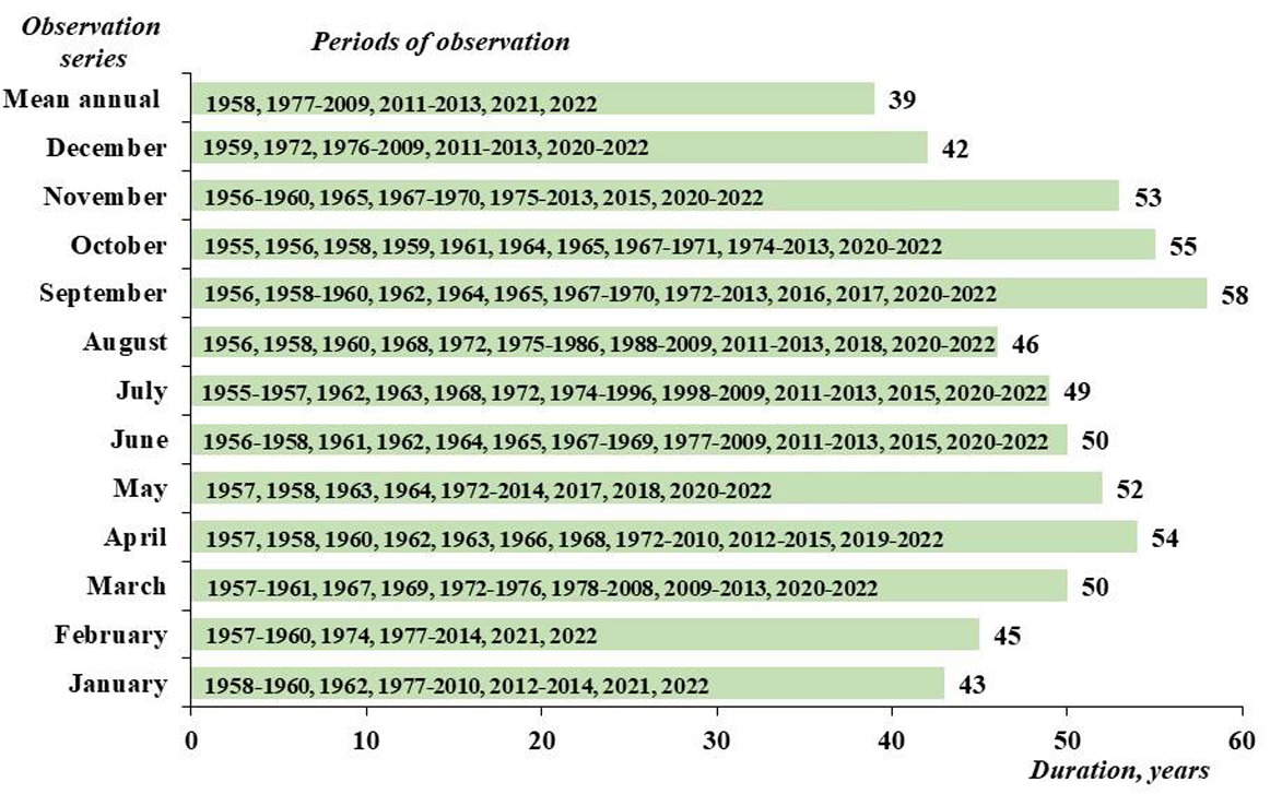
During the observation period, the mean annual values of NSW speed ranged from 3.5 to 6.1 m/s. The multi-annual NSW speed is 4.8 m/s. The highest multi-annual mean monthly NSW speed was observed in September (6.0 m/s), and the lowest in January (3.6 m/s). The lowest mean monthly value of NSW speed was observed in June 1997 (1.7 m/s), and the highest in October 1955 (9.3 m/s).
3.2. Statistical analysis
Applying the four statistical tests at the 1% level of significance to assess the homogeneity of mean annual values of NSW speed in the area of the Vernadsky Station showed that all of the annual values indicated a violation of homogeneity in 1998, when the values of their statistics exceeded the critical values (Table 1). Therefore, the series of mean annual values of NSW speed in the area of the Vernadsky Station is inhomogeneous. Along with this, however, the tests indicate homogeneity of mean monthly values, which did not exceed critical values of the statistics of two or more tests for any month of year (Table 2). Thus, the series of mean monthly values is homogeneous, but the series of mean annual values is inhomogeneous. This is a contradictory result.
Table 1.
Results of tests of homogeneity of mean annual near-surface wind speed in the area of the Vernadsky Station according to statistical tests at the 1% level of significance.
| Test | The value of statistic | Critical value | Year of disturbance of homogeneity | p-value |
|---|---|---|---|---|
| Alexandersson | 14.9 | 11.2 | 1998 | 0.0009 |
| Buishand | 2.01 | 1.76 | 1998 | 0.0003 |
| Pettitt | 271 | 251 | 1998 | 0.0008 |
| von Neumann | 1.30 | 1.33->2.00 | - | 0.0000 |
Table 2.
Results of testing homogeneity of mean monthly near-surface wind speed in the area of the Vernadsky Station according to statistical tests at the 1% level of significance
In addition, the tests show years in which trends in the mean monthly NSW speeds possibly change. However, for most months, the years of change, according to various tests, do not coincide, a finding that also fails to illuminate the multi-year NSW speed trends. For example, in February, the year of change is 2001, according to the Buishand test, and 1998 according to the Pettitt test. It can be assumed that such ambiguous results depend on the properties, features, and characteristics of the statistical tests themselves and result from the different durations of observation series with their many missing records (Figs. 2, 3).
The Mann-Kendall test was one of the tests used to assess the stationarity of the NSW speed series at the Vernadsky Station. The analysis of results shows that significant trends at the 1% level are found for only two series, namely, mean monthly values for February and mean annual values (Table 3). The mean annual values series is non-stationary, while the mean monthly values series from which this series is calculated is stationary. This result is also illogical and contradictory, like the previous finding obtained from the assessment of homogeneity of the series of NSW speed observations.
Table 3.
Results of tests of stationarity of the near-surface wind speed series according to the Mann-Kendall test at a significance level of 1%, the Vernadsky Station.
In general, when evaluating record homogeneity and stationarity, difficulties arise with the interpretation of results, since it is impossible to unambiguously establish the long-term tendencies and changes. That is why homogeneity and stationarity were further assessed by graphic methods.
3.3. Graphical analysis
The chronological graph of the mean annual NSW speed shows a turning point in 1998, which confirms the inhomogeneity and non-stationarity of this series according to statistical tests (Fig. 4, Tables 1, 3). At the same time, the mass curve shows that the cumulative values do not deviate from a straight line, which indicates homogeneity of mean annual NSW speed (Fig. 5).
Fig. 4.
Chronological graph of the mean annual near-surface wind speed in the area of the Vernadsky Station.
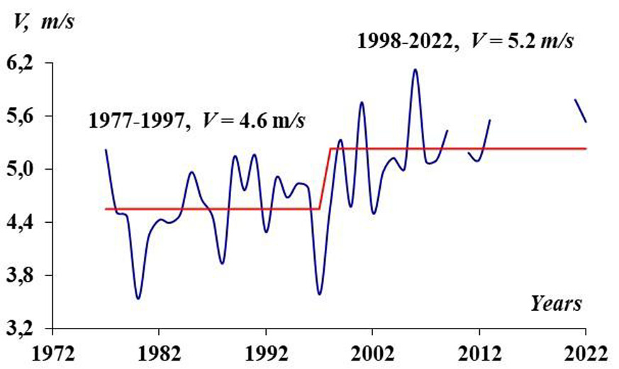
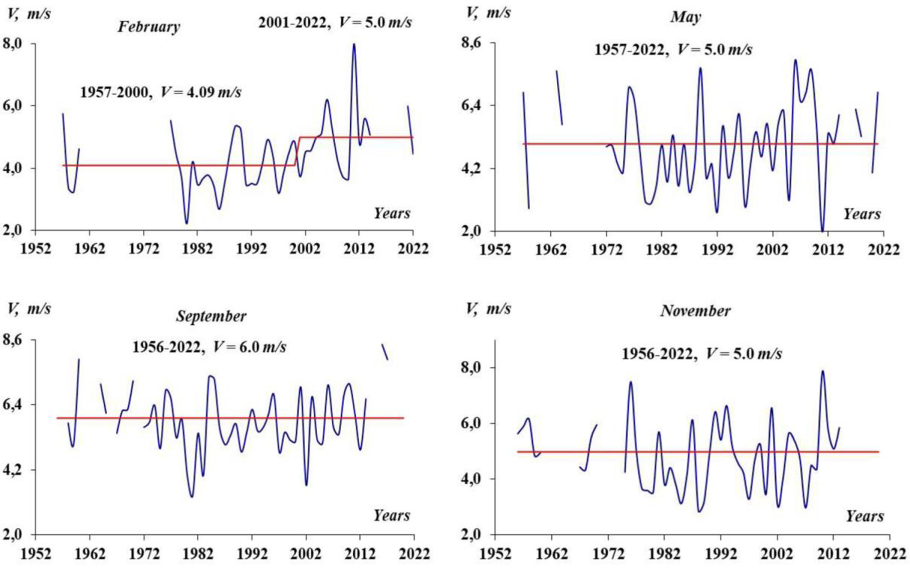
Fig. 5.
Chronological graphs of the mean monthly values near-surface wind speed for individual months in the area of the Vernadsky Station.
Analysis of the residual mass curve of mean annual NSW speed showed that in 1998, there was a transition from a decrease to an increase (Fig. 5). At the same time, the beginning of the decreasing phase cannot be clearly determined by the residual mass curve of the mean annual NSW speed, since there are many missing records. Similarly, it is impossible to determine the end of the increasing phase, which continues to the present.
According to the graphical analysis, the mean monthly series are mostly homogeneous and stationary. The chronological graphs of the mean monthly NSW speed thus show no changes in the observation series, except for the month of February (Fig. 5).
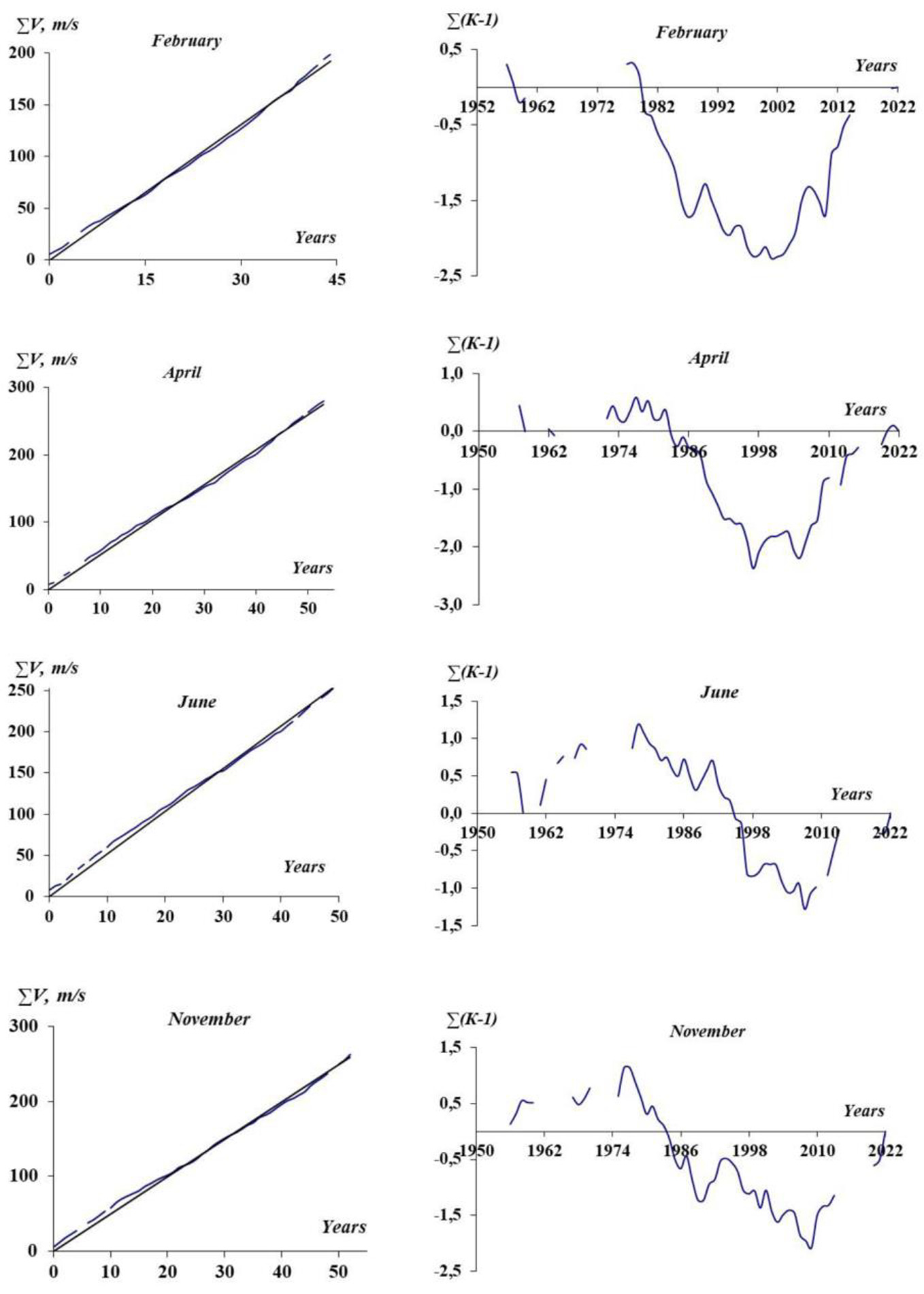
This result coincides with the results obtained by statistical tests (Tables 1, 2). At the same time, the mass curves of monthly NSW speed do not show deviations from a straight line, which indicates the homogeneity of these series of observations (Fig. 6 – left). The residual mass curves of mean monthly NSW speed indicate short- and long-term cyclical fluctuations (Fig. 6 – right). Non-stationarity of the mean monthly series for February, which is the same as for the mean annual observation series (per the Mann-Kendall statistical test, Table 3), is only due to the decreasing and increasing phases of long-term cyclic fluctuations (Fig. 6). Therefore, the February series is quasi-stationary. The observation series for other months are stationary because they contain both decreasing and increasing phases, as well as the final or initial phases of adjacent cycles. In all months of the year, there has been a tendency of an increasing near-surface wind speed at the Vernadsky Station during the past 20 years.
4. Discussion
Even at the end of the 19th century, the German scientist Eduard Brückner studied the cyclical fluctuations of the climate and proposed the 35-year-long Brückner cycle of cold, damp weather alternating with warm, dry weather in northwestern Europe (Stehr, Storch 2000). Throughout the 20th century, research into hydrometeorological quantities’ fluctuations and changes over time was conducted using various approaches and methods. Many investigations have shown that short- and long-term cycles of different durations are observed in time series of atmospheric precipitation, air temperature, and river flow throughout the world (Gorton 1931; Karl 1988; Pekárová et al. 2003; Nidzgorska-Lencewicz, Czarnecka 2019; dos Santos et al. 2023).
Our study shows that NSW speeds, both mean annual and mean monthly, in the area of the Vernadsky Station have short- and long-term cyclical fluctuations (Figs. 5, 7). Pekárová et al. (2003) reported that in the different phases of cyclic fluctuations of hydrometeorological characteristics, there are observed tendencies that have different signs. So, the decreasing phase has values of hydrometeorological parameters significantly lower than the values observed in the increasing phase. This pattern results in differences in the mean values for these phases of cyclic fluctuations. Therefore, an observation series that has only decreasing and increasing phases of long-term cyclical fluctuations is classified as non-homogeneous and non-stationary by the statistical tests. This is exactly the result obtained by the statistical tests for the observation series of the mean annual and February mean monthly NSW speeds in the area of the Vernadsky Station. At the same time, this result is influenced by a short series of observations, since the series of observations in other months are longer and partially cover the adjacent cycles of long-term cyclical fluctuations. The observation series of the mean annual and February mean monthly NSW speeds have both decreasing and increasing phases, although these series are unfinished (i.e., they continue). So, such series must be classified as quasi-stationary. That is why, for such series, it is important to periodically repeat the analyses. A combined application of statistical and graphic methods, as we have applied here, will support more reliable estimates of homogeneity, stationarity, and tendencies of observation series.
5. Conclusions
At the Vernadsky Station, measurements of NSW speed were checked for missing records (e.g., those resulting from mechanical problems). The analysis showed that a significant part of the data contains errors, and these may be especially relevant for some years. Subsequently, incorrect data were removed from the study. Thus, new series of statistically reliable data for mean annual and mean monthly NSW speeds for the period 1955-2022 were generated. As a result of this data editing, the series obtained for individual months were of different durations.
For example, the resulting series for September had the longest duration (58 years), and the series of annual mean NSW speed had the shortest duration (39 years).
The series of mean annual and February mean monthly NSW speeds are quasi-homogeneous and quasi-stationary since they only have the phases of decrease and increase for long-term cyclic fluctuations. The other series of NWS speed observations are homogeneous and stationary. Where the Vernadsky NWS speed series lack homogeneity and stationarity, according to statistical tests, it is caused by comparing the different phases of cyclic fluctuations (i.e., decreasing and increasing phases), which have different statistical characteristics.
During the past 20 years at the Vernadsky Station, according to the residual mass curves, NSW has an increasing tendency in all months of the year. Similar results were obtained in several previous papers (Turner et al. 2009; Dong et al. 2020; Andres-Martin et al. 2024). The multi-annual NSW speed is 4.8 m/s. The highest multi-annual mean monthly NSW speed was observed for September (6.0 m/s), and the lowest was observed for January (3.6 m/s).
We emphasize that using a combination of statistical approaches as applied in this analysis allows more robust results and could be applied to other hydrometeorological variables or characteristics.