1. Introduction
Global warming as a result of greenhouse gas emissions is now undeniable, and there has been a significant increase in the atmospheric concentration of CO2 over the last century (Alemu, Dioha 2020). The increase in average and extreme temperatures in Africa can be attributed to climate change caused by human activity (Trisos et al. 2022). Several studies have found that temperatures are changing in Africa. Muthoni et al. (2019) studied the extent and significance of spatio-temporal trends in rainfall, maximum (Tmax) and minimum (Tmin) temperatures for West Africa. In northern Ghana, De Pinto et al. (2012) found that temperatures were higher than in any other part of Ghana and that they could increase between 1.0°C and 3.0°C by 2060 and between 1.5°C and 5.2°C by 2090. In Mali, Kouressy et al. (2019) report that between 1951 and 2010, maximum temperatures increased significantly by 0.44°C to 1.53°C and minimum temperatures by 1.05°C to 1.93°C, depending on the location. In Benin, Senegal, and Niger, mean annual minimum temperature increased significantly between 1965 and 2013: in less than 50 years, minimum temperature increased by 1.2°C in Djougou (Benin), 1.8°C in Bambey (Senegal) and 1.4°C in Niamey (Niger) (Kosmowski et al. 2015).
Few statistical studies have been carried out in Burkina Faso on the trend and variability of extreme temperature (Bambara et al. 2018; Rouamba et al. 2023), and even fewer on the seasonal analysis of extreme temperature in the Sudano-Sahelian part of Burkina Faso. It is very important to gain a better understanding of the seasonal occurrence of extreme temperatures because they cause illness and even death in young children and the elderly (Arisco et al. 2023). In this article, seasonality is based on rainfall, as temperatures change before, during, and after the rainy season. Three periods can be distinguished: the pre-wet period (January to May), the wet period (June to October) and the post-wet period (November to December). In this study, we analyze the seasonal trends in extreme temperatures over the past few decades.
2. Materials and methods
2.1. Data and methods
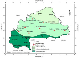
Burkina Faso is located in West Africa, where Sahelian, Sudano-Sahelian, and Sudanian climatic domains dominate (Fig. 1).
The raw data used to assess extreme temperatures came from NASA’s POWER (National Aeronautics and Space Administration Prediction of Worldwide Energy Resource) online public database (https://power.larc.nasa.gov/data-access-viewer). Power data are based on satellite observations from which surface insolation values are derived. The meteorological parameters are based on the MERRA-2 assimilation model. The database has the advantage of being generally continuous over time and is based on a global grid with a resolution of 0.5° latitude by 0.5° longitude (Marzouk 2021). Numerous studies have assessed the accuracy of the data and found that the source of the data (NASA POWER) is sufficiently accurate to allow valid interpretation (Jiménez-Jiménez et al. 2021; Marzouk 2021; Ahmed et al. 2022; Kwawuvi et al. 2022; Oloyede et al. 2023; Darman et al. 2024; Kheyruri et al. 2024).
Data for Burkina Faso from NASA’s power data access viewer was collected at monthly intervals over the period 1981 to 2022. The characteristics of the localities selected are shown in Table 1 below (Table 1).
Table 1.
Characteristics of the selected stations, all within the Sudan-Sahelian.
[i] Source: https://power.larc.nasa.gov/data-access-viewer/.
2.1.1. Statistical normality and homogeneity
The normality test is important for determining appropriate methods for the assessment of significant trends in time series of precipitation data, using parametric or non-parametric methods of trend analysis (Talib et al. 2024). Normality tests, including Shapiro-Wilk W, Anderson-Darling, Lilliefors, and Jarque-Bera tests, were applied to the annual time series to evaluate the normal distribution of time series data. For all four tests, the null hypothesis is as follows:
H0: the temperature time series has a normal distribution; if the p-value is less than 5%, the normal distribution can be rejected, and the alternative hypothesis (H1) can be accepted. Among the tests proposed, the Shapiro-Wilk and Anderson-Darling tests are considered the most accurate, while the Lilliefors and Jarque-Bera tests are given for reference (Hammer 2024). Only the first two tests have been considered in this study. Thus, the mathematical formula for the calculation of Shapiro-Wilk (W) is (Asamoah, Ansah-Mensah 2020):
where xi is the value of the ordered sample, ai is a constant generated from the means, variances and covariances of the ordered statistics, n is the number of observations, and
The Anderson-Darling (AD) test uses the cumulative distribution function to determine normality, and its formula is as follows (Asamoah, Ansah-Mensah 2020):
where n is the sample size, F(x) is the cumulative distribution function for the specified distribution, and i the ith sample for an ascending order.
The Buishand test was used to determine the homogeneity of the temperature data. The Buishand test, like the Petitt test, is more sensitive to breaks in the middle of the time series. (Wijngaard et al. 2003). In the Buishand test, the assumption is that the data are normally distributed and that the data are independently and randomly distributed (Bickici Arikan, Kahya 2019). The adjusted partial sums are defined as (Lin et al. 2015):
There will be no systematic deviation of
The Von Neumann test (VNT) examines the randomness and change point detection of the time series. The VNT test statistic can be computed as (Lebeza et al. 2023):
where N is the test static value of VNT, X is observed time-series data and
2.1.2. Method of trend analysis
Trends in hydro-climatological variables are generally evaluated using a variety of statistical tests, such as linear regression, Mann-Kendall (MK) and modified MK tests, with non-trending pre-whitening and Sen Slope (SS) estimators (Xu et al. 2007; Longobardi, Villani 2010; Nisansala et al. 2020; Ay 2021); other authors add the Spearman’s r test (Yue et al. 2002; Yacoub, Tayfur 2019). The Mann-Kendall test, Spearman’s r test and Sen’s slope estimator were used to assess the trend and magnitude of seasonal temperature extremes in Burkina Faso.
• Linear Regression Analysis.
Linear Regression is a parametric method used to estimate linear trends in time series (Rahmani et al. 2015; Esit, Yuce 2022):
where Y is the temperature time series, X is the year or time, β0 = Intercept, β1 = Slope, and ε is the residual error.
• Mann-Kendall Trend Test.
Mann-Kendall (MK) is a non-parametric test (Mann 1945). It is specifically used to detect trends in environmental, climatic, and hydrological time series (Aditya et al. 2021; Lornezhad et al. 2023). According to Ahmad et al. (2015), the null hypothesis (H0) of this test is that there is no monotonic trend in the time series. The alternative hypothesis (Ha) is that there is a trend. The MK test is based on the calculation of the variance (S) and is obtained by the following equation (Mirabbasi et al. 2020):
The sgn function is calculated as follows:
where n is the length of the sample, xk and xj come from k = 1, 2, ..., n – 1 and j = k + 1, ..., n. If n is greater than 8, the S statistic approximates the normal distribution. The mean of S is 0 and the variance of S can be obtained as follows:
The Z statistic is calculated using the formula:
The null hypothesis H0 (no trend) is rejected if the significance level or p-value is <5%. Table 2 below shows the level of significance.
Table 2.
Interpretation of the meaning of the trend in the MK.
| Mann-Kendall test (p-value) | Significance of the trend |
|---|---|
| <0.01 | Very significant |
| 0.01≤ p <0.05 | Significant |
| ≥0.05 | Not significant |
• Spearman’s r Test (SR).
Spearman’s r (SR) is a powerful method for detecting linear and non-linear trends and is frequently used to test for the absence of trends (Rahman et al. 2017). In this test, the null hypothesis (H0) of the test is that all the data in the time series are independent and identically distributed, while the alternative hypothesis (H1) is that there are upward or downward trends. Positive values of the SRZ standardized test statistic indicate upward trends, while negative values indicate downward trends in the time series (Zakwan 2021). The test statistics rsp and standardized statistics Zsp are defined as (Ahmed et al. 2022):
where Di is the rank of ith observation, I is the chronological order number, n is the total length of the time series data, and Zsp is Student’s t-distribution with (n − 2) degree of freedom. The positive values of Zsp represent an increasing trend across the hydrologic time series, and negative values represent the decreasing trends.
• Sen’s slope estimator test.
The non-parametric Sen test (Sen 1968) is commonly used for the estimation of the magnitude of trends in time series data. The Sen test for the slope assumes a linear trend and is a quantification of the change over time (Muia et al. 2024). The slope of Sen is calculated according to the following equation (Frimpong et al. 2022):
where, xj and ik = the data values at times j and k (j > k).
If there is only one datum in each period, then:
where n = total number of observations.
The N values of Qi have been ranked from the lowest to the highest, and the median slope or Sen’s slope estimator has been calculated as follows:
A positive value of Qi represents an upward trend; a negative value of Qi represents a downward trend, over time (Ahmad et al. 2015).
2.1.3. Method analysis variability
• The moving average method
The moving average is the most widely used method for the measurement of seasonal fluctuations (Bacescu-Carbunaru, Condruz-Bacescu 2013). In this study, moving averages (MA) have been used for the assessment of the overall trend in the variation of extreme temperatures (Zeitoun 2024):
where n is the number of data points, d is the moving average, and M is the data calculated as the simple moving average with the period is 3, MA: moving average.
• The Fligner Killeen test
This non-parametric test (Conover et al. 1981) indicated significant differences in variability by testing the equality of the coefficients of variation of two samples. The coefficient of variation (or relative variation) is defined as the ratio of standard deviation to the mean in percent, and is computed as (Hammer 2024):
The null hypothesis of the statistical test is H0: the samples were taken from populations with the same coefficient of variation. However, when the p-value is less than 5%, the null hypothesis is rejected, and the alternative hypothesis is supported.
• Temperature Anomaly Detection Method
Anomaly detection is a popular research area in time series data mining, where data points that don’t conform to other data are referred to as anomalies (Wickramasinghe et al. 2023). Z-score is used to detect temperature anomalies, so the hypothesis is that the temperature data either contain anomalies or they do not (Zeitoun 2024). The formulas for a z-score transformation are (Jackson 2009):
where z is the symbol for the standard score, µ is the mean, σ is the standard deviation. The significant level is 0.95, with alpha (α) equal to 0.05, and the critical value of the Z-score is +1.96 and –1.96 (Zeitoun 2024). According to Pandey et al. (2023), the value of the z-score indicates the number of standard deviations the variables are from the mean. If a z-score is equal to 0, then the mean is on the mean. A positive z-score indicates that the raw score is comparatively higher than the mean and a negative z and a negative z-score indicates that the raw score is lower than the mean.
3. Results
3.1. Statistical normality and homogeneity in the study area
Table 3 below shows that the maximum temperature data for Ouahigouya, Diapaga, Dédougou, Ouagadougou, Kaya, and Kouka sites are normally distributed. On the other hand, the Shapiro-Wilk and Anderson-Darling statistics imply a lack of normality in the minimum temperature data.
Table 3.
The normality of extreme temperature data.
The temperature data (maximum, minimum) were also subjected to homogeneity tests. The Buishand test shows that there is a change in both the maximum and minimum temperature data. The Von Neumann test was also applied to the temperature data. Table 4 shows the results of the two homogeneity tests.
Table 4.
Homogeneity of extreme temperature data.
Table 4 shows that temperature data change with the seasons. The change in maximum temperature data occurred in 2000 in Diapaga during the rainy season. In Kaya, the changes occurred before, during and after the rainy season in 1998, 2006, and 2010 respectively. In Ouahigouya, the change occurred during the pre-rainy season, as it did at Fada Gourma and Boromo. In Ouagadougou and Dédougou, however, the changes affected both the pre-rainy season and the rainy and post-rainy seasons. Overall, there has been an increase in maximum temperatures following the changes that occurred between 1998 and 2010. However, there has been very little change in the minimum temperature data. In Diapaga and Fada Gourma, the minimum temperature data were disrupted, especially during the wet and humid pre-season in 2004 and 1992 in Diapaga.
In Fada Gourma the change occurred in 1998. The minimum temperature increased significantly in the following years.
3.2. Statistical trends in extreme temperatures in the Sudano-Sahelian zone of Burkina Faso
3.2.1. Analysis of maximum temperature trends using linear regression methods
The results of the normality test revealed that the maximum temperature data are normally distributed , allowing for trend analysis using parametric tests, particularly linear regression. The table below shows the seasonal trends over the period 1981-2020 (Table 5).
Table 5.
Trends in maximum temperatures over the period 1981-2022.
3.2.2. Minimum temperature trends using Mann-Kendall and Spearman’s r tests and Sen’s slope estimator
The minimum temperature trend time series data were examined using the Mann-Kendall (MK), Spearman’s r and Sen (SS) slope tests, as the results of the normality test indicated that these data are not normally distributed, requiring non-parametric tests for trend analysis.
• Mann-Kendall trend test and Sen’s estimator of the slope
Table 6 below shows that, on the whole, the extreme temperatures at the different sites studied do not show any trend in the temperature series. However, in Diapaga, Kouka, Fada Gourma, and Dédougou, positive trends were observed in the period before the rainy season. On the other hand, negative trends before and during the rainy season were observed in Ouahigouya and Kaya
Table 6.
Trends and amplitudes of minimum temperatures between 1981 and 2022.
• Spearman’s r test
This test was also applied to the temperature data. It was found that the pre-wet season (January to May) shows positive trends, with positive correlation coefficients for maximum and minimum temperatures in Diapaga, Kaya, Ouahigouya, Ouagadougou, Kouka, Fada Gourma, Boromo and Dédougou. During the rainy season, the trend in extreme temperatures is also upward in all the locations studied, with a very high degree of significance. However, the minimum temperatures in Boromo and Dédougou show no trend between 1981 and 2022. On the other hand, in the period after the rainy season, temperature trends are significant over the period 1981-2022.
Table 7.
below gives details by season and month of the extreme temperature trends over the period 1981-2022.
3.3. Extreme temperature variability in the Sudano-Sahelian domain of Burkina Faso
In this study, the variability of extreme temperatures was analyzed by moving averages, the anomaly method, and the Fligner-Killeen test.
3.3.1. Analysis of variability in extreme temperatures using moving averages and Fligner-Killeen test
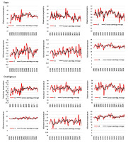
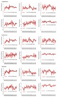
The moving averages show a fluctuating trend in extreme temperatures, reflecting the variability of the time series from 1981 to 2022. Overall, there is a four-stage trend in maximum temperatures, with a decrease between 1981 and 1998, an increase between 1999 and 2001, a decrease between 2022 and 2011, and an increase between 2012 and 2022. However, the behavior of minimum temperatures is different. There is no phase of change, but rather a continuous sawtooth pattern. This means that the variability of minimum temperatures is even greater than that of maximum temperatures. The stations close to the Sahelian domains (Ouahigouya, Kaya) and the Sudanian domains (Kouka, Boromo) have strong fluctuations in minimum temperatures, compared with the stations in Ougadougou, Fada Gourma, and Diapaga, which are in the center of the Sudano-Sahelian zone. Figure 2 shows the changes in temperature variability between 1981 and 2022 for the selected study regions. In the northeast region, the Kaya station was chosen. Similarly, in the north and central regions, the Ouahigouya and Ouagadougou stations were chosen because of their different variation. The Dédougou station in the Boucle du Mouhoun region was chosen because the other stations (Boromo, Kouka) are similar in terms of temperature variation. The same is true for the Fada Gourma station in the eastern region.
These variations are quite large in comparison with the pre-rainy season, the rainy, and the post-rainy season (Table 8).
Table 8.
Comparative variability of extreme temperatures for the periods before the rainy season, during the rainy season and after the rainy season.
3.3.2. Analysis of anomalies as a factor in temperature variability in Burkina Faso
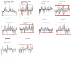
Extreme temperatures are anomalies that develop decade by decade over the period 1981 to 2022. Indeed, in the 1980s, especially in 1981, 1982, 1983, and 1987, extreme temperature anomalies (maximum, minimum) exceeding z = 1.96 were recorded during the pre-rainy season at all the sites studied. Further temperature anomalies occurred in 1994, 1995, and 1998, mainly during the rainy and post-rainy seasons. From 2000 onward, the occurrence of extreme temperature anomalies increased significantly: the number of years in which anomalies occurred increased over the period 2000-2022, with anomalies occurring in 2000, 2001, 2002, 2003, 2005, 2009, 2011, 2013, 2015, 2019, and 2021. Extreme temperature anomalies occur during the rainy season, the post-rainy season and, to a lesser extent, the pre-rainy season. This indicates an increase in temperature variability at the study sites. Figure 3 shows temperature anomalies from 1981 to 2022.
4. Discussion
4.1. Temperature trends in Burkina Faso and Africa
The results of the study are quite remarkable. Extreme temperatures (maximum and minimum) show a change in the 2000s compared to the period 1981-2022 period. Furthermore, extreme temperatures show an upward trend according to Spearman’s r, regardless of seasonality. Temperature variability was also strong and increasing over the period 2000-2022. However, the trends vary from station to station. This could be explained by a general variation in rainfall and temperature across the country. Indeed, the area occupied by the Sahelian and Sudano-Sahelian domains has increased over time (1931-2010) to the detriment of the Sudanese domain (Rouamba 2017). Furthermore, isotherms have also shifted from north to south from 1971 to the present day, reflecting temperature dynamics across the country (Dipama 2014). Yaméogo and Rouamba (2023) also found an increase and change in maximum temperatures in the Sahelian, Sudano-Sahelian, and Sudanese domains over the period 1960-2019. Other studies in the Sudano-Sahelian domain (Rouamba et al. 2023) found similar results. Yanogo and Yaméogo (2023) also note that temperatures in the Sudano-Sahelian region of Burkina Faso are changing, particularly in the 2000s over the period 1990-2020. Several other studies carried out in West Africa and Africa as a whole corroborate the results of this study. For example, Sanogo et al. (2023) found that maximum temperatures in Mali are increasing, but that the trend was also upward for the period 1991-2020. Similar studies have confirmed the findings of previous studies. For example, Musa et al. (2021) found an increasing trend and high variability in extreme temperatures in north-central Nigeria. Other studies conducted in Nigeria (Ogunrayi et al. 2016; Ekwueme, Agunwamba 2021; Dan’azumi, Ibrahim 2023), Mauritania (Yacoub, Tayfur 2019), Senegal (Djaman et al. 2017) and Gambia (Jabbi et al. 2021) have made similar observations. According to Ilori and Ajayi (2020), extreme temperatures are evolving due to temporal breaks in temperature data in the 1980s, which then show an upward trend until 2010. Other regions of Africa are affected by changes in seasonal temperature cycles. In East Africa, particularly Ethiopia and South Africa, extreme temperatures are increasing (Worku et al. 2022; Chapungu et al. 2024). The same trends have also been observed in Central Africa, such as the Democratic Republic of Congo (Posite et al. 2024) and Burundi (Niyongendako et al. 2020). The work of Umeh et al. (2024) on 48 African countries shows an overall trend toward rising temperatures in all countries except Madagascar and Niger.
4.2. Seasonal temperature variability in Burkina Faso and West Africa
Maximum and minimum temperatures show inter-seasonal variability in the eight (08) stations in the Sudano-Sahelian region. This could be explained by the fact that in the arid tropical region of Africa where Burkina Faso is located, temperature is modulated by rainfall. Thus, the temperature is very high as the rainy season approaches, then moderately high during the rainy season, and the temperature drops just after the rainy season, i.e., in November, December, and January. This situation could influence the seasonal variability of extreme temperatures. In addition, in other studies in Burkina Faso, Yaméogo and Rouamba (2023), and Koala et al. (2023a), add that seasonal variability in maximum temperatures is observed across the country. Koala et al. (2023b) predict that a continuous trend in temperature variability in the Sudano-Sahelian zone (from the Nakambè catchment) will continue until 2050. Studies carried out in West Africa confirm these results. In Nigeria, maximum, minimum, and mean temperatures in the Niger basin over the period 1948-2008 (Oloruntade et al. 2016), as well as in the coastal region of Nigeria (Agbonaye, Okonofua 2024), have been rising steadily. In Mali and northern Togo they increased over the period 1951-2010 (Kouressy et al. 2019l; Gadedjisso-Tossou et al. 2021). According to Ringard et al. (2016) and Asamoah and Ansah-Mensah (2020), there has been an increase in extreme variability across the West African region (Sahel and Gulf of Guinea). There has also been an increase in extreme temperature anomalies. The various results show a general increase in temperatures, interspersed with a high-temperature variability according to season (wet and dry). This seasonal temperature variability results from the hydrological cycle (Diba et al. 2022).
5. Conclusion
Temperature extremes in the Sudano-Sahelian region of Burkina Faso were analyzed using normality, homogeneity, trend, and anomaly statistics. The normality tests showed that the maximum temperature data generally followed a normal distribution, while the minimum temperature data did not follow a normal distribution. Homogeneity tests of the temperature data reveal temperature breaks in the 2000s before, during, and after the rainy season for maximum temperature data. However, minimum temperatures showed little change. The study shows that temperatures change seasonally, with maximum temperatures changing more markedly than minimum temperatures during the pre-rainy season, the rainy season, and the post-rainy seasons. Temperatures are also highly variable, with anomalies observed in the pre-rainy season, the rainy season, and the post-rainy season in the 2000s. Local and regional authorities must, therefore, take urgent action to protect vulnerable groups.


